Figure
1.
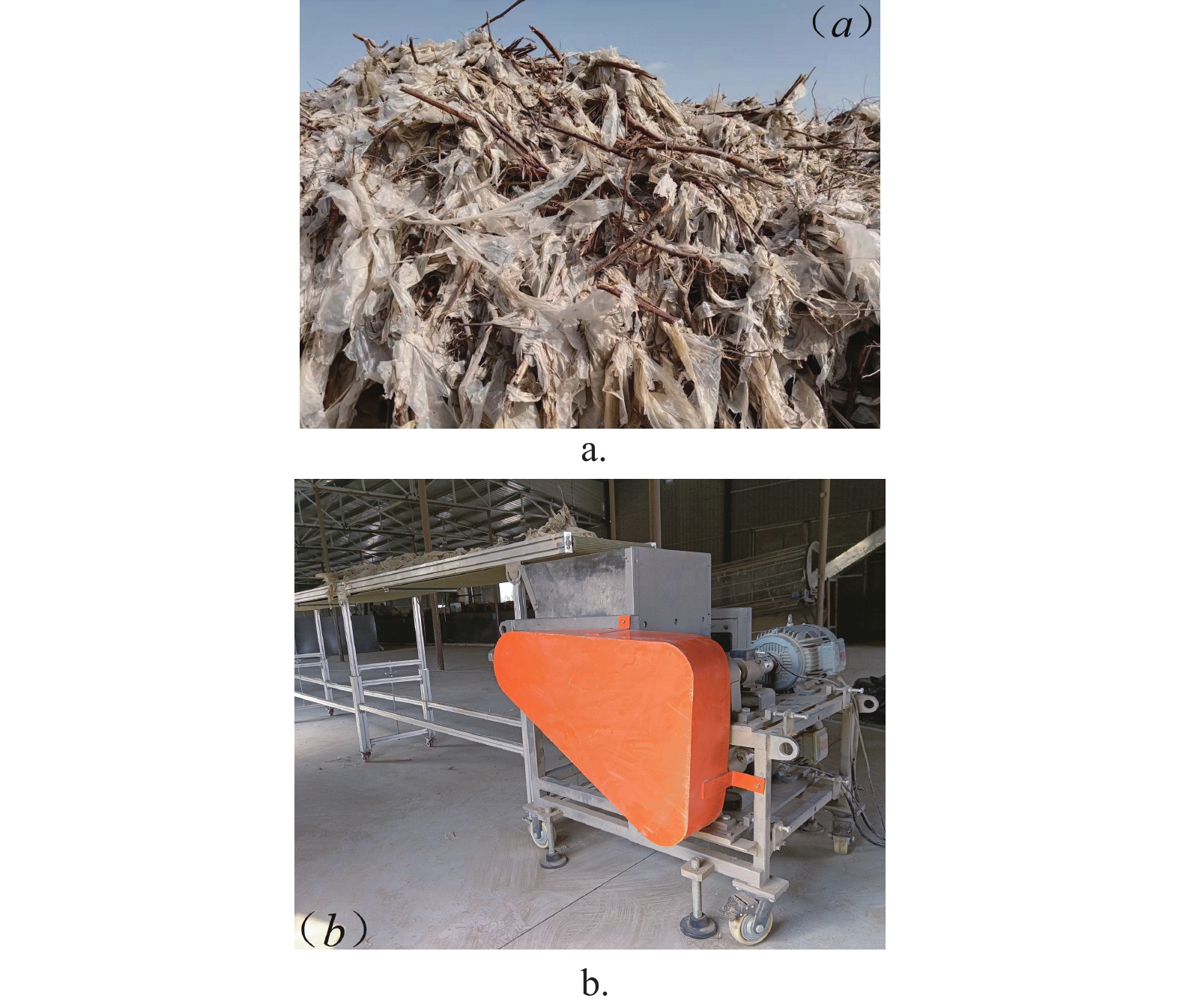
RF and impurities (a) and cutting device (b)

| Citation: |
Liang R Q, Wu G D, Jia R, Meng H W, Tai R J, Jia H P, et al. Influence law on the effect of shredding characteristics of residual film in the mixture of mechanically recovered residual films and impurities in cotton fields. Int J Agric & Biol Eng, 2025; 18(1): 51–63. DOI: 10.25165/j.ijabe.20251801.8508

|
Few studies have been carried out on special shredding technology and equipment, hence it is hard to find out the characteristic rule of distribution of residual films after shredding. By evaluating the mechanical properties of the residual film during the cutting process of a mixture of mechanically recovered residual film and impurities, the main parameters influencing the film distribution feature were acquired. Physical tests were conducted on the basis of a multi-blade toothed shredding device. A relationship model between the film distribution feature and main parameters was constructed through the central grouping method and regression analysis of variance, aiming to investigate the influence rule of main parameters on the film distribution feature and the interaction between them, and to obtain the optimal combination of parameters for the cutting device. The difference between the experimental validation value and the model prediction ranged from 1.03% to 9.56%, which showed that the model has reliable and accurate predictive ability.
Mulching film is a petroleum-based long-chain polyethylene plastic product[1,2]. When left too long in the field, some intermolecular covalent bonds of the polymer could break and the molecular chain could be invalid[3], causing aged and fractured films which are hard to recover. Xinjiang is a major cotton production base in China. Due to the continuous cropping with mulching technology in this area, the residual mulch in the cotton field is 1.5-5.0 times higher than China’s residual mulch standard (75 kg/hm2)[4], and soil and environmental pollution are particularly serious[5,6]. Mechanical recovery technology has become a trend and an important means for recovery of residual films (RF)[7], and has initially solved the problem of RF pollution. However, the recovered residue is usually mixed with a large amount of cotton straws, soil, and other impurities, which would eventually form a mixture of mechanically recovered RF and impurities in cotton fields (MRI)[8]. Different from urban wastes or other agricultural wastes, MRI (Figure 1a) features an unstable structure, different mixture proportions, disordered distribution of film-soil-straw, strong adhesion of film and soil, and intertwined film and straw, which has increased the initial cleaning cost of RF and extended the production period. This has hindered the resource utilization process of RF to a certain extent and has reduced the quality of recycled products.
As energy recovery and utilization of waste plastics could cause waste of resources[9], resource recovery and utilization has become a definite trend to treat waste plastics and has attracted global attention for its great development potential[10,11]. The RF in MRI is such a recyclable waste plastic resource[12]. Reasonable and suitable recovery, primary cleaning, and resource utilization not only can relieve environmental pollution, improve resource utilization, and reduce resource exploitation cost[13-15], but also can solve the RF pollution effectively and environmentally. Therefore, it is urgent to carry out studies with regards to primary cleaning technology of MRI to form an organic circular economy involving the recovery, treatment, and resource utilization of MRI.
To realize the resource utilization of MRI in Xinjiang, the study on primary cleaning technology mainly focused on the separation technology of MRI[16], and the shredding technology and equipment development require further enrichment. Shredding technology is a primary process in waste treatment[9], which not only acts as the precondition for mixture separation but also significantly affects the follow-up process, quality of recycled products, and economic benefits after primary treatment[17]. Restricted by technological condition, processing mode, and market orientation, current resource utilization of RF in Xinjiang cotton fields is still quite simple, and is mainly wash granulating[18]. According to surveys, in order to satisfy the actual production need and ensure the cleaning effect and quality of recycled products, MRI is usually separated manually and then the separated residues are shredded by waste plastic shredder. Waste plastic shredder can shred residues with low levels of impurities, but it is not appropriate for direct shredding of MRI. Based on the characteristics of RF and cotton straws[8], researchers developed a differential roller cutting device with a multi-blade tooth cutter as the core, solving the direct shredding problem of MRI (Figure 1b). Related works have shown that it is a challenge to obtain the influence rule of critical parameters of the cutting equipment on the material distribution properties[17,19,20].
Consequently, by analyzing the stress characteristics of the RF in MRI, a mechanical model of the RF was developed and the main parameters affecting the distribution feature of the RF were obtained. Simultaneously, physical experiments were carried out with a multi-blade toothed shredding device of mixed materials collected during the mechanized harvesting of cotton fields. The model of the relationship between the distribution feature of the RF and the main parameters of the cutting device (e.g., number of teeth, rotational speed, and cutters gap) were obtained by analyzing the experimental results with the analysis of variance method. Then the significance of the main parameters influencing the RF distribution feature was investigated to reveal the rule of residue shredding characteristics of MRI. The objective of this study is to provide some theoretical foundation and technique support for the study of MRI shredding technology and the relevant shredding device development[8].
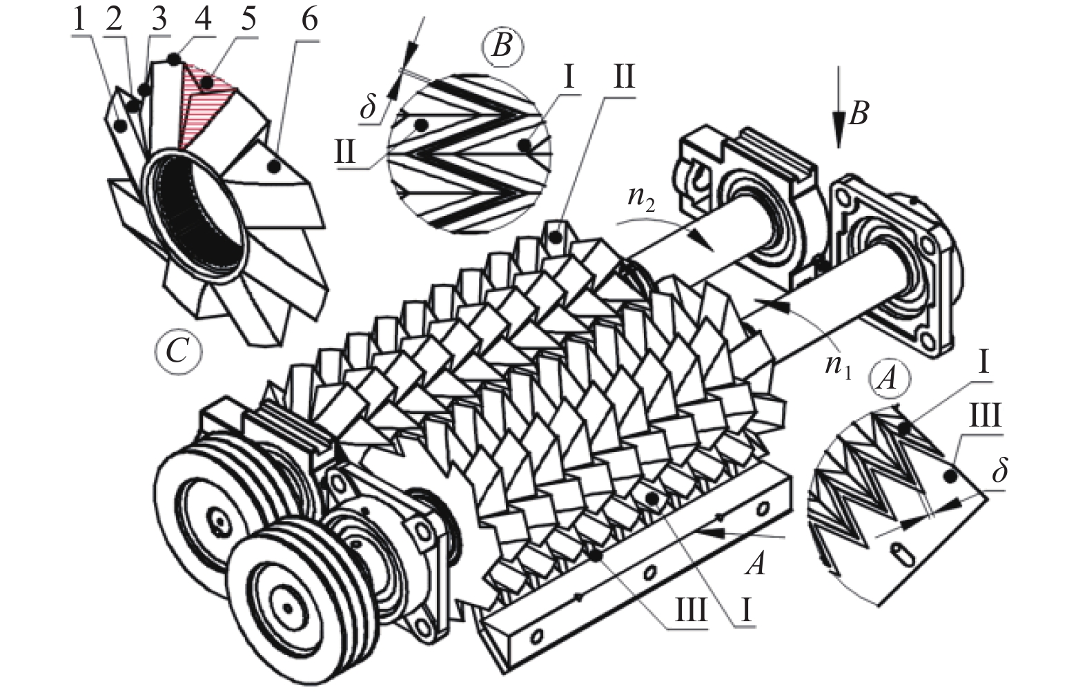
In Figure 2, the high-speed cutter (H-cutter) and low-speed cutter (L-cutter) are shown as the core parts of the shredding device[8]. The cutter parts mainly consist of the rake face of tooth, back blade, side face of tooth, top blade, back blade, and V-shaped area. During the shredding process, H-cutter, L-cutter, and stationary cutter (S-cutter) interact with each other to realize the compression, cutting, and stretching of the RF. The purpose of this section is to analyze the force characteristics of the RF layer under the interaction condition between H-cutter, L-cutter, and S-cutter and investigate the influence rule of dynamic properties of the RF during the cutting process of MRI, as well as to determine the crucial factors of RF dynamic properties.
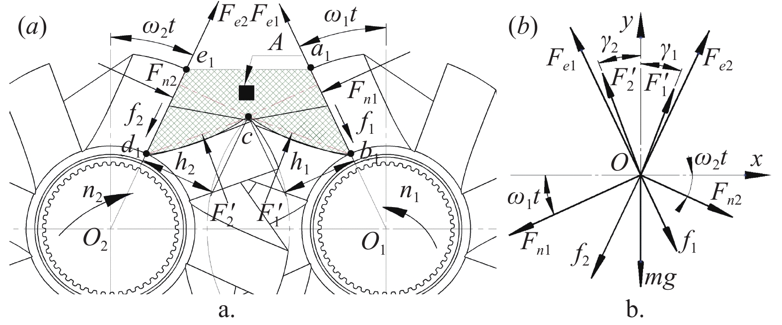
A single layer of RF is usually very thin (nominal film thickness: 0.01 mm), but has high ductility and flexibility, and is usually fluffy and compressible in MRI. Starting from the rake face of H-cutter and L-cutter which coincides with the positive direction of the y-axis, when H-cutter and L-cutter turn ω1t and ω2t separately, the acting forces that cause the compression and deformation of the RF layer mainly include the compressing force (Fn1, Fn2), the frictional force (f1, f2), and the support force of the back blade face (F1, F2), etc. To analyze the force characteristics of the RF layer during the compressing process, the RF layer unit A was taken as the object of study in this part[8]. It is assumed that the support force (F1, F2) is simplified to the plane stress (F′1, F′2) of a plane perpendicular to the y-axis, which projects on the line connecting point ac (point ec), and remains perpendicular to the line connecting points ac (ec).
The simplified diagram of the force characteristics of the constructed RF layer unit A is shown as Figure 3b. The equilibrium equation of the RF layer unit A on the x-axis and y-axis is:
| {F′2sinγ2+Fn1cosω1t+f2sinω2t+Fe1sinω1t=F′1sinγ1+Fn2cosω2t+f1sinω1t+Fe2sinω2tF′1cosγ1+F′2cosγ2+Fe1cosω1t+Fe2cosω2t=mg+Fn1sinω1t+Fn2sinω2t+f1cosω1t+f2cosω2t | (1) |
where, F′1 and F′2 are the support forces of the side blade face of H-cutter and L-cutter on the RF layer unit, separately, N; γ1 and γ2 are the included angles of the support forces F′1 and F′2 with the positive direction of the y-axis, separately, (°); m is the mass of the RF layer unit, kg; g is the gravity acceleration, m/s2; Fn1 and Fn2 are the compressing forces produced by the elastic deformation of the RF layer unit when compressed by the rake face of H-cutter and L-cutter, separately, N; ω1t and ω2t are the turning angles of H-cutter and L-cutter, separately, (°); f1 and f2 are the frictional forces between the rake face of H-cutter and L-cutter with the RF layer unit, separately, N; Fe1 and Fe2 are the centrifugal forces of the rake face of H-cutter and L-cutter to the RF layer unit, separately, N.
In Equation (1), the included angles γ1 and γ2 of the forces F′1 and F′2 with the positive direction of the y-axis are:
| {γ1=arctanrcosα1−r′cosω1trsinα1−r′sinω1tγ2=arctanrcosα2−r′cosω2trsinα2−r′sinω2t | (2) |
There is a certain function between the compressing forces Fn1 and Fn2 with the material properties and compression height. When the rake face of the cutters compresses the RF layer, the vertical distance h from the point c to the rake face is assumed as the compression height to be compressed. As the multi-blade toothed cutter is a rotational working part, the compressing forces Fn1 and Fn2 are the resultant forces of the x-axis and y-axis compressing forces, separately, which can be expressed by:
| {Fn1=EcA′r√cos2ω1th2x+sin2ω1th2yFn2=EcA′r√cos2ω2th2x+sin2ω2th2yf1=μcFn1;f2=μcFn2; μc=tanμkFe1=mω21r;Fe2=mω22r | (3) |
where, Ec is the elastic modulus of RF layer, MPa; A′ is the stressed area of the RF layer unit, m2; hx, hy are the original heights of the RF layer unit at the x-axis and y-axis, separately, which are ranged from 0~rsinα to 0~(r-rcosα), m; μc is the coefficient of friction between RF and cutters; μk is the friction angle between RF and cutters, (°); ω1, ω2 are the angular velocities of H-cutter and L-cutter, separately, rad/s.
Substituting the friction and centrifugal force equations of (3) into (2), the F′1 and F′2 are:
| {F′1=m[gsinγ2+ω21rsin(ω1t−γ2)−ω22rsin(ω2t+γ2)]sin(γ1+γ2)+Fn1cos(γ2+ω1t+μk)−Fn2cos(ω2t−γ2+μk)sin(γ1+γ2)cosμkF′2=m[gsinγ1+ω22rsin(ω2t−γ1)−ω21rsin(ω1t+γ1)]sin(γ1+γ2)+Fn2cos(ω2t+μk−γ1)−Fn1cos(γ1+ω1t+μk)sin(γ1+γ2)cosμk | (4) |
According to model (4), when the material properties, the top blade radius r, and the tooth hub radius r′ are constant, the support force has a certain function with the angular velocity ω1 of H-cutter and the angular velocity ω2 of L-cutter. When the RF layer is compressed completely to a certain degree, it is cut by the interactive force between H-cutter and L-cutter. Due to the speed discrepancy between H-cutter and L-cutter[8], the rake faces of the two cutters interact with the top blade and back blade to cut the RF layer. Therefore, the mechanical properties and established mechanical model of the RF layer unit under the interactive conditions between the rake face with the top blade and the back blade of H-cutter and L-cutter, separately, will be studied in the next part[8].
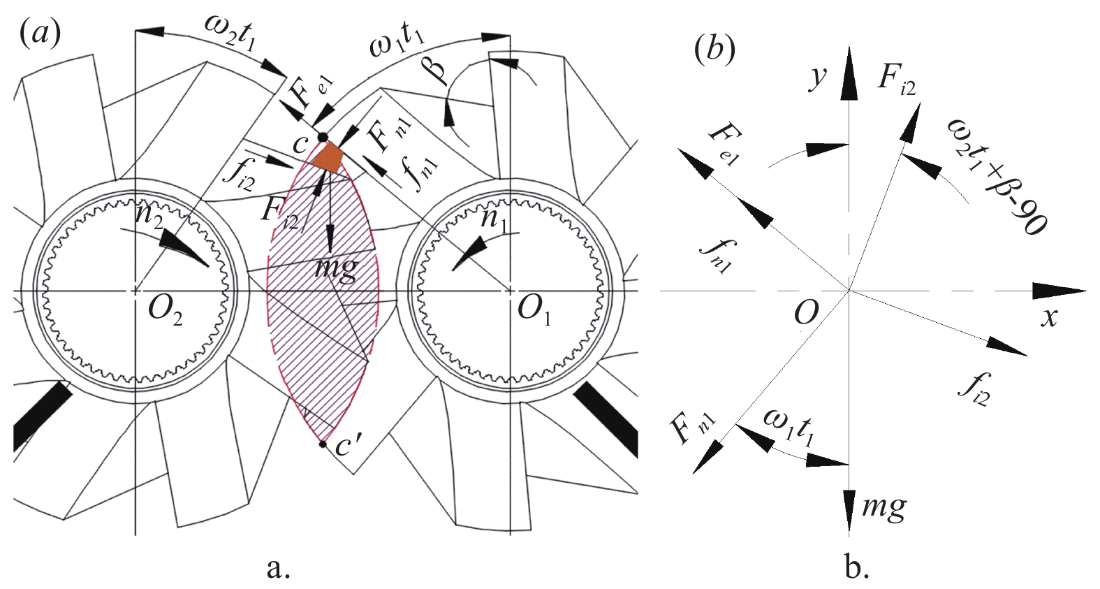
In Figure 4a, at the t1 moment, the rake face of H-cutter interacts with the back blade of L-cutter to cut the compressed RF layer[8]. The external forces exerted on the RF layer unit mainly include the centrifugal force Fe1 formed by the rotation of H-cutter, the support force Fn1 and the frictional force fn1 of the rake face of the cutters, as well as the cutting force Fi2 and the frictional force fi2 of the back blade of L-cutter. The simplified force characteristics of the RF unit are shown as Figure 4b.
The equilibrium equation of the RF layer unit on the x-axis and y-axis is:
| {Fi2sin(ω2t1+β−90)+fi2cos(ω2t1+β−90)(Fe1+fn1)cosω1t1+Fn1sinω1t1=Fi2cos(ω2t1+β−90)+(Fe1+fn1)sinω1t1=mg+Fn1cosω1t1+fi2sin(ω2t1+β−90) | (5) |
where, Fi2 is the cutting force of the back blade of L-cutter on the RF unit, N; Fe1 is the centrifugal force of H-cutter on the RF unit, N; Fn1 is the support force of the rake face of H-cutter on the RF unit, N; fi2 is the frictional force produced from the relative motion between the back blade of L-cutter and the RF layer unit, N; fn1 is the frictional force between the rake face of H-cutter, N; ω1t1 and ω2t1 are the turning angles of H-cutter and L-cutter, separately, (°); β is the angle between the rake face and back blade of the cutters, (°).
By substituting the friction and centrifugal force equation of (3) into model (5), the results of Fn1 and Fi2 are acquired:
| {Fn1=mcosμk[ω21rsin(ω2t1+β+μk−ω1t1)−gcos(ω2t1+β+μk)]cos(ω1t1+ω2t1+β+2μk)Fi2=mcosμk[gsin(ω1t1+μk) - ω21rcosμk]cos(ω2t1+β−ω1t1) | (6) |
According to Equation (6), when the radius r of the cutters, the included angle β, and the frictional coefficient of the RF and cutters are all constant, the cutting force Fi2 and support force Fn1 on the RF layer produced by the interaction between the rake face of H-cutter and the back blade of L-cutter have a certain function with the rotational speed of H-cutter and L-cutter.
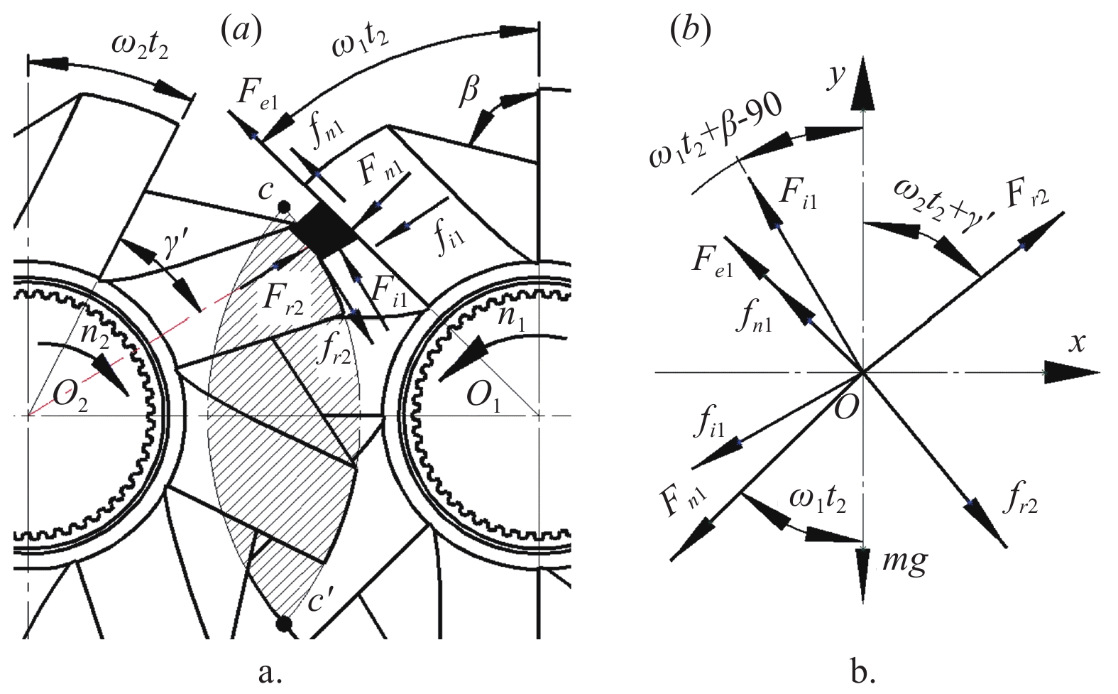
Figure 5a shows the force characteristics of the RF layer at the time t2 under the interactive condition between the rake face and top blade of the cutters. At this time, the RF layer unit mainly receives the support forces Fn1 and Fi1 and the frictional forces fn1 and fi1 produced by the rake face and back blade of H-cutter. Meanwhile, the RF layer unit also receives the centrifugal force Fe1 produced by the rotation of H-cutter. In comparison with H-cutter, the main forces on the RF layer unit from L-cutter mainly include the cutting force Fr2 and frictional force fr2 of the top blade. The simplified force analysis diagram of the residual unit is shown as Figure 5b.
The equilibrium equation of the RF layer unit on the x-axis and y-axis is:
| {Fr2sin(ω2t2+γ′)+fr2cos(ω2t2+γ′)=Fi1sin(ω1t2+β−90)+(Fe1+fn1)cosω1t2+fi1cos(ω1t2+β−90)+Fn1sinω1t2Fr2cos(ω2t2+γ′)+Fi1cos(ω1t2+β−90)+(Fe1+fn1)sinω1t2=fr2sin(ω2t2+γ′)+fi1sin(ω1t2+β−90)+Fn1cosω1t2+mg | (7) |
where, fi1 and fn1 are the frictional forces of the rake face and back blade of H-cutter with the RF unit, separately, N; Fr2 is the cutting force of the top blade of L-cutter on the RF layer unit, N; Fn1 and Fi1 are the support forces of the rake face and back side blade of H-cutter on the RF unit, N; Fe1 is the centrifugal force of H-cutter on the RF unit, N; fr2 is the frictional force between L-cutter and RF layer unit, N; ω1t2 and ω2t2 are the turning angles of H-cutter and L-cutter, (°); γ′ is the deviation angle of the connecting line between the force bearing point of the RF layer unit and the rotating center to the rake face of the cutters at ω1t2, (°).
Substituting the friction and centrifugal force equation of (3) into (7) yields Fi1 and Fr2 as follows:
| {Fi1=mcosμk[ω21rcos(ω2t2+γ′+μk−ω1t2)−gsin(ω2t2+γ′+μk)]cos(ω1t2+β+ω2t2+γ′+2μk)−Fn1sin(ω2t2+γ′−ω1t2)cos(ω1t2+β+ω2t2+γ′+2μk)Fr2=mcosμk[gcos(ω1t2+β+μk)−ω21rsin(2ω1t2+β+μk)]cos(ω2t1+γ′+ω1t2+β+2μk)+Fn1cos(2ω1t2+β+2μk)cos(ω2t1+γ′+ω1t2+β+2μk) | (8) |
According to Equation (8), when the radius r of the cutters, the included angle β, and the frictional coefficient between RF and the cutters is constant, there is a certain function between the cutting force Fr2 and the support force Fi1 with the rotational speed of H-cutter and L-cutter.
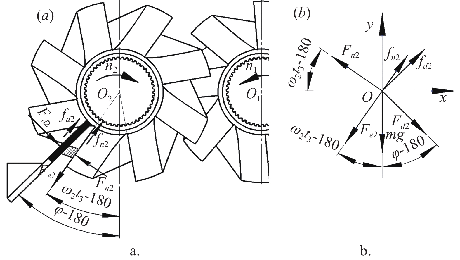
According to the analysis of stretching and tearing characteristics of RF, the longer RF that was not cut thoroughly would intertwine with the cutters. To avoid such a problem, S-cutter was set under H-cutter and L-cutter, which can also cut the RF while preventing intertwining. Due to the same interactive features between S-cutter and H-cutter or L-cutter, the force characteristics of the RF layer under the interactive condition between the rake face of L-cutter and S-cutter were investigated, and the influence rule of the RF dynamic properties was explored[8].
Assume that at time t3, the turning angle of the rake face of L-cutter against the positive direction of the y-axis is ω2t3, as shown in Figure 6a. Except for the gravity, the RF layer also received other external forces, e.g. the centrifugal force Fe2 produced from the rotation of L-cutter, the support force Fn2 and the frictional force fn2 of the cutters rake face, and the support force Fd2 and frictional force fd2 of the S-cutter. Meanwhile, the back blade of the cutters near the S-cutter is also ranged in the phase angle [π, 2π]. It is assumed that no support force or frictional force are produced from the back blade of the cutters on the RF layer unit. The simplified analysis diagram of the force characteristics of the RF layer unit is shown as Figure 6b.
The equilibrium equation of the RF layer unit on the x-axis and y-axis is shown as Equation (9):
| {Fd2sin(φ−180)+fd2cos(φ−180)+fn2sin(ω2t3−180)=Fn2cos(ω2t3−180)+Fe2sin(ω2t3−180)Fn2sin(ω2t3−180)+fn2cos(ω2t3−180)+fd2sin(φ−180)=Fd2cos(φ−180)+mg+Fe2cos(ω2t3−180) | (9) |
where, Fd2 and Fn2 are the support forces of the S-cutter and the rake face of the cutters on the RF layer unit, separately, N; fd2 and fn2 are the frictional forces, N; Fe2 is the centrifugal force of the cutters on the RF layer unit, N; φ is the position angle clockwise of the S-cutter to the positive direction of the y-axis, (°); ω2t3 is the turning angle of L-cutter relative to the positive direction of the y-axis, (°).
Substituting the centrifugal force equation of (3) into (9), the acting forces of Fd2 and Fn2 are obtained as follows:
| {Fn2=mcosμk[gsin(φ+μk)−ω22rsin(ω2t5+φ+μk)]cos(ω2t5+2μk+φ)Fd2=mcosμk[gcos(ω2t5+μk)−ω22rcosμk]cos(ω2t5+2μk+φ) | (10) |
According to Equation (10), when the cutters, S-cutter, and RF material are at a certain level, there is a certain function between the acting forces Fn2 and Fd2 and the angular velocity ω2 of L-cutter.
In conclusion, when cutting MRI with staggered H-cutter and L-cutter, the change rule of the dynamic properties of RF is related to the rotational speed n1 of H-cutter and the speed discrepancy Δn between H-cutter and L-cutter[8]. Meanwhile, relevant studies show that the tooth number and the gap also have an effect on the distribution feature of materials after shredding[17,21-23]. Due to the complicated structural characteristics of MRI, the cotton straws also affect the distribution feature of RF after shredding. Therefore, the influence rule of the main parameters on the distribution feature of RF in MRI after shredding was obtained through physical tests on the basis of RF dynamic properties analysis.
The experiments were conducted in the middle of October 2022 at the Key Laboratory of Northwest Agricultural Equipment, Ministry of Agriculture and Rural Affairs, Shihezi University. The test materials were obtained from Tuan Chang cotton field near Shihezi, Xinjiang. The materials were collected in late September 2022, shown in Figure 1a. The instruments and devices used in the test process in this paper are consistent with the reference [8].
During the shredding of MRI, the particle size of soil-dominated bulk material is small and easily causes dust pollution, so it should be removed before the test. During the test, the MRI was first deposited uniformly on the infeed conveyor belt[24]. The cutting device was started and the infeed conveyor belt was opened as the cutting device was stabilized. Due to the large volume and fluffy nature of MRI, overfeeding or excessive speed can cause the shredding device to become clogged, leading to overloads and momentary shutdowns. Therefore, the machining quantity for each group of materials and the feeding speed were set as 2.0±0.1 kg and 0.01 m/s based on the preliminary tests[8]. After the test, the crossover method was used on samples with reference to GB/T26551-2011. The sample mass of each group was 400±10 g. After sampling, the RF was manually selected from the MRI, and the total mass of the RF was recorded as m. Meanwhile, to reveal the influence rule of the maximum outer scale distribution feature of the RF in the MRI, the ratio between the RF mass within each range of the maximum outer dimension and the total RF mass was counted.
Combined with the theoretical analysis results in Section 2, and considering the structural characteristics of the shredding device, the value range of these parameters of the tooth number of cutters z (a), gap between the teeth and from S-cutter δ (b), rotation speed of H-cutter n1 (c), and speed discrepancy of H-cutter and L-cutter Δn (d) were determined. A four-factor, five-level central combination test scheme was designed using the Central Composite Design module of Design Expert data processing software[8]. Each test group was repeated three times. The test protocol and results are listed in Table 1.
| No. | a | b | c | d | x1/% | x2 /% | x3/% | x4/% |
| 1 | –1 (6) | –1 (2 mm) | –1 (800 r·min–1) | –1 (–400 r·min–1) | 5.68±1.52 | 16.29±3.06 | 59.56±3.09 | 18.47±3.87 |
| 2 | 1 (10) | –1 | –1 | –1 | 2.45±0.88 | 18.15±7.28 | 57.42±6.26 | 21.98±10.42 |
| 3 | –1 | 1 (4 mm) | –1 | –1 | 2.67±0.55 | 17.91±4.21 | 67.49±4.06 | 11.93±6.65 |
| 4 | 1 | 1 | –1 | –1 | 4.56±1.48 | 18.99±7.04 | 64.37±5.07 | 12.08±4.08 |
| 5 | –1 | –1 | 1 (1000 r·min–1) | –1 | 3.19±1.88 | 18.16±10.10 | 60.80±8.15 | 17.85±6.88 |
| 6 | 1 | –1 | 1 | –1 | 2.87±1.47 | 23.65±17.64 | 54.36±18.35 | 19.12±18.24 |
| 7 | –1 | 1 | 1 | –1 | 1.85±0.25 | 16.54±4.04 | 70.19±3.94 | 11.42±3.94 |
| 8 | 1 | 1 | 1 | –1 | 2.43±0.53 | 14.61±5.37 | 66.78±7.06 | 16.18±10.24 |
| 9 | –1 | –1 | –1 | 1 (–200 r·min–1) | 5.44±2.20 | 11.84±6.10 | 59.12±6.29 | 23.60±2.80 |
| 10 | 1 | –1 | –1 | 1 | 2.13±0.67 | 14.61±8.60 | 62.93±9.99 | 20.33±14.99 |
| 11 | –1 | 1 | –1 | 1 | 2.02±0.58 | 20.82±3.78 | 44.65±5.76 | 32.51±8.47 |
| 12 | 1 | 1 | –1 | 1 | 1.57±0.29 | 12.78±5.88 | 40.49±3.53 | 45.16±6.23 |
| 13 | –1 | –1 | 1 | 1 | 3.36±1.99 | 18.26±6.16 | 59.75±8.25 | 18.63±9.31 |
| 14 | 1 | –1 | 1 | 1 | 1.45±0.43 | 18.31±5.36 | 64.69±6.69 | 15.55±3.23 |
| 15 | –1 | 1 | 1 | 1 | 1.65±0.88 | 14.13±5.78 | 59.02±2.36 | 25.2±6.78 |
| 16 | 1 | 1 | 1 | 1 | 1.47±0.28 | 9.16±3.11 | 56.52±5.70 | 32.85±3.93 |
| 17 | –2 (4) | 0 (3 mm) | 0 (900 r·min–1) | 0 (–300 r·min–1) | 4.39±2.16 | 18.78±7.67 | 62.57±6.50 | 14.26±8.91 |
| 18 | 2 (12) | 0 | 0 | 0 | 2.11±1.15 | 17.25±7.65 | 63.51±11.98 | 17.13±8.29 |
| 19 | 0 (8) | –2 (1 mm) | 0 | 0 | 2.97±1.14 | 24.15±7.79 | 60.82±3.12 | 12.06±10.20 |
| 20 | 0 | 2 (5 mm) | 0 | 0 | 1.33±0.32 | 21.66±11.70 | 56.25±6.44 | 20.76±6.02 |
| 21 | 0 | 0 | –2 (700 r·min–1) | 0 | 4.58±2.29 | 12.83±8.18 | 56.55±8.09 | 26.04±12.03 |
| 22 | 0 | 0 | 2 (1100 r·min–1) | 0 | 1.58±0.59 | 10.17±4.59 | 61.15±7.31 | 27.10±8.99 |
| 23 | 0 | 0 | 0 | –2 (–500 r·min–1) | 2.68±0.96 | 12.56±8.66 | 60.55±7.87 | 24.21±10.74 |
| 24 | 0 | 0 | 0 | 2 (–100 r·min–1) | 1.62±0.63 | 5.14±2.54 | 45.58±13.75 | 47.66±15.84 |
| 25 | 0 | 0 | 0 | 0 | 1.57±0.89 | 18.78±4.25 | 56.83±4.80 | 22.82±8.07 |
| 26 | 0 | 0 | 0 | 0 | 2.60±0.42 | 18.90±6.79 | 55.55±4.91 | 22.95±7.20 |
| 27 | 0 | 0 | 0 | 0 | 1.75±0.36 | 20.02±4.34 | 59.38±5.64 | 18.85±8.18 |
| 28 | 0 | 0 | 0 | 0 | 2.19±0.64 | 17.39±3.47 | 62.10±8.04 | 18.32±6.75 |
| 29 | 0 | 0 | 0 | 0 | 2.34±0.40 | 19.58±13.17 | 55.76±5.54 | 22.32±13.61 |
| 30 | 0 | 0 | 0 | 0 | 2.22±0.64 | 15.04±7.17 | 61.91±8.89 | 20.83±15.38 |
 DownLoad:
CSV
DownLoad:
CSV
During the separation process, the material size and distribution applicable to different separation technology instruments were significantly different[25]. Preliminary field investigations showed that overlength RF or cotton straws could increase the probability of intertwined materials, which was regarded as the major cause of the low efficiency of separating MRI. Therefore, to reduce the maximum outside dimension of the RF to meet the working requirements, different separation technologies such as electrostatic method, air separation, and suspension method should be used[23,26]. But because small RF may lead to microplastic pollution, excessive cutting of the films should also be avoided[27]. Referring to the statistical range of shredded waste plastics in the literature[9], the RF was classified according to the maximum outer dimensions of [0, 20) mm, [20, 100) mm, [100, 500) mm, [500, ~) mm based on the specific separation demands and the primary cleaning status of RF. The calculation of the ratio of RF mass to total RF mass of different maximum outside dimension distribution ranges is shown as Equation (11):
| x1=m1m×100%;x2=m2m×100%;x3=m3m×100%;x4=m4m×100% | (11) |
where, m, m1, m2, m3, and m4 are the mass of the total mass and maximum outside dimension of the RF samples at the ranges of [0, 20) mm, [20, 100) mm, [100, 500) mm and [500, ~) mm, separately, g. x1, x2, x3, and x4 are the ratio of m1, m2, m3, and m4 to m, %.
The analytical results are shown as Table 2. According to the results of regression variance analysis of the test response index x1, the p values of the odd factors a, b, c, d and the interaction term ab were all much smaller than 0.01, which were the extreme influence factors on x1. The p values of the interaction terms of ad, a2, and c2 ranged from 0.01-0.05, which were found to be significant influence factors on x1. The p values of the interaction terms of ac, bc, bd, cd, b2, and d2 were all higher than 0.05, and the effect on x1 value was not significant. The order of the extremely significant factors and significant factors of the significance of p value to x1 was: c>ab>b>a>d>a2>c2>ad.
| Source | x1 | x2 | x3 | x4 | ||||||||||
| F-Value | p-value | F-Value | p-value | F-Value | p-value | F-Value | p-value | |||||||
| Model | 8.66 | <0.0001** | 11.21 | <0.0001** | 10.04 | <0.0001** | 14.19 | <0.0001** | ||||||
| a | 18.1 | 0.0007** | 0.63 | 0.4392 | 0.67 | 0.4257 | 3.6 | 0.0771 | ||||||
| b | 18.54 | 0.0006** | 5.17 | 0.0381* | 1.8 | 0.1995 | 10.1 | 0.0062** | ||||||
| c | 27.84 | <0.0001** | 0.21 | 0.6535 | 11.08 | 0.0046** | 3.07 | 0.0999 | ||||||
| d | 10.45 | 0.0056** | 21.33 | 0.0003** | 37.89 | <0.0001** | 72.39 | <0.0001** | ||||||
| ab | 23.15 | 0.0002** | 12.01 | 0.0035** | 1.45 | 0.2477 | 4.49 | 0.0512 | ||||||
| ac | 2.2 | 0.1588 | 0.02 | 0.8906 | 0.026 | 0.8734 | 0.037 | 0.8495 | ||||||
| ad | 4.68 | 0.0471* | 5.79 | 0.0294* | 2.4 | 0.1424 | 0.11 | 0.7407 | ||||||
| bc | 0.41 | 0.5322 | 23.4 | 0.0002** | 9.89 | 0.0067** | 0.049 | 0.8277 | ||||||
| bd | 1.84 | 0.1952 | 0.089 | 0.7694 | 55.16 | <0.0001** | 43.57 | <0.0001** | ||||||
| cd | 0.66 | 0.4296 | 0.068 | 0.7976 | 7.05 | 0.018* | 5.44 | 0.034* | ||||||
| a2 | 8.57 | 0.0104* | 0.16 | 0.6962 | 5.65 | 0.0312* | 7.95 | 0.013* | ||||||
| b2 | 0.1 | 0.7566 | 16.74 | 0.001** | 0.064 | 0.8034 | 6.36 | 0.0234* | ||||||
| c2 | 6.37 | 0.0233* | 20.45 | 0.0004** | 0.16 | 0.6934 | 2.85 | 0.1122 | ||||||
| d2 | 0.1 | 0.7566 | 42.55 | < 0.0001** | 5.41 | 0.0345* | 31.01 | <0.0001** | ||||||
| Lack of fit | 2.61 | 0.1506 | 0.85 | 0.6121 | 0.81 | 0.6409 | 3.12 | 0.1106 | ||||||
| R2=0.8899;R2adj=0.7871;C.V=21.01% | R2=0.9127;R2adj=0.8313;C.V=10.48% | R2=0.9036;R2adj=0.8135;C.V=4.72% | R2=0.9298;R2adj=0.8643;C.V=14.4% | |||||||||||
| Notes: ** refers to extremely significant factor (p≤0.01), *refers to significant factor (0.01<p≤0.05),p>0.05 refers to non-significant factor. | ||||||||||||||
DownLoad:
CSV
For the test response index x2, the p values of the odd factor d with the interaction terms ab, bc, b2, c2, and d2 were all much smaller than 0.01, which were the extreme influence factors on x2. The p values of the odd factor b with the interaction term ad were all between 0.01 and 0.05, which were significant influence factors on x2. The p values of the odd factors a and c with the interaction terms of ac, bd, cd, and a2 were all higher than 0.05, and the effect on x2 value was not significant. According to the significance of p value to x2 value, the extremely significant factors and significant factors were: d2>bc>d>c2>b2>ab>ad>b.
The results for the test response index x3 show that the p values of the odd factors c and d with the interaction terms bc and bd were all much smaller than 0.01, which were the extreme influence factors on x3. The p values of the interaction terms cd, a2, and d2 were all between 0.01 and 0.05, which were the significant influence factors on x3. The p values of the odd factors a and b with the interaction terms of ab, ac, ad, b2, and c2 were all higher than 0.05, and the effect on x3 value was not significant. According to the significance of p value to x3 value, the extremely significant factors and significant factors were: d>bd>c>bc>cd>a2>d2.
The results for the test response index x4 show that the p values of the odd factors b and d with the interaction terms bd and d2 were all much smaller than 0.01, which were the extreme influence factors on x4. The p values of the interaction terms cd, a2, and b2 were all between 0.01 and 0.05, which were significant influence factors on x4. The p values of the odd factors a and c with the interaction terms of ab, ac, ad, bc, and c2 were all higher than 0.05, and the effect on x4 value was not significant. According to the significance of p value to x4 value, the extremely significant factors and significant factors were: d>bd>d2>b>a2>b2>cd.
As shown in Table 2, the model coefficients’ p values of X1, X2, X3,and X4 were much smaller than 0.01, which indicate the extreme significance of the second-order response models. The determination coefficients R2 of models X1, X2, X3, and X4 were 0.8899, 0.9127, 0.9036, and 0.9298, separately. The adjusted determination coefficients R2adj were 0.7871, 0.8313, 0.8135, and 0.8643, separately. These results indicate a good explanation of the four models, which can make precise and robust predictions of the test response indices of x1, x2, x3, and x4.
The quadratic response surface regression models X1, X2, X3,and X4 were established as Equation (12):
| {X1=2.11−0.48a−0.48b−0.59c−0.36d+0.66ab+0.2ac−0.3ad+0.088bc−0.19bd+0.11cd+0.31a2+0.033b2+0.27c2+0.033d2X2=18.29−0.28a−0.8b−0.16c−1.63d−1.5ab+0.061ac−1.04ad−2.1bc+0.13bd−0.11cd+0.13a2+1.35b2−1.5c2−2.16d2X3=58.59−0.46a−0.76b+1.89c−3.49d−0.83ab−0.11ac+1.08ad+2.18bc−5.16bd+1.84cd+1.26a2+0.13b2+0.21c2−1.23d2X4=21.02+1.22a+2.05b−1.13c+5.49d+1.67ab−0.15ac+0.27ad−0.17bc+5.21bd−1.84cd−1.7a2−1.52b2+1.02c2+3.36d2 | (12) |
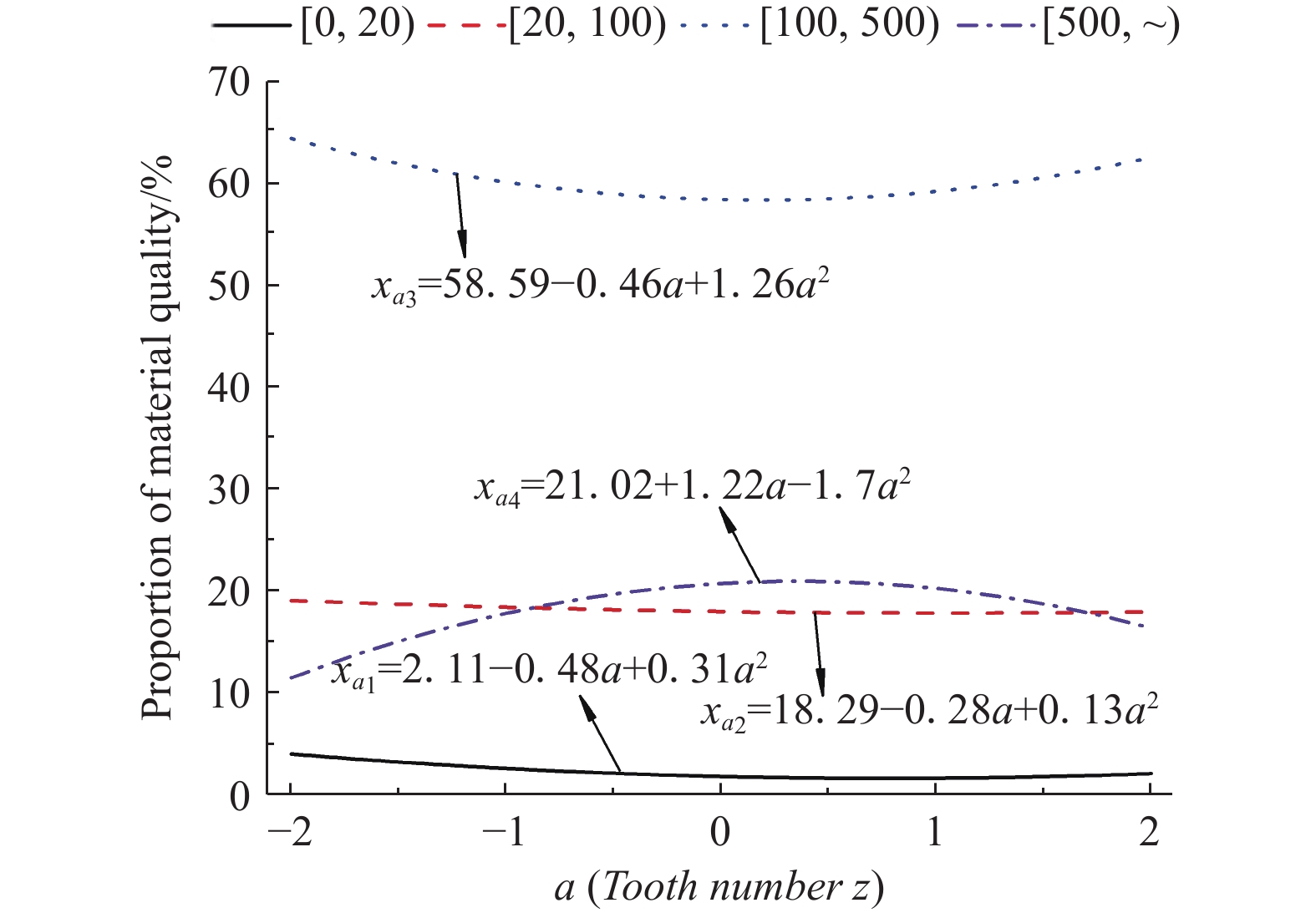
In Figure 7, when tooth number z rose from 4 to 8, the curves xa1, xa2 and xa3 all showed a decreasing trend, while xa4 showed an increasing trend, and the decreasing trend of xa3 and the increasing trend of xa4 were obvious. As tooth number z increased, the rake face, back blade, and V-shaped area increased, while the top blade arc length became shorter[8]. The increase of the area of rake face and back blade strengthened the interaction of the rake face and back blade between H-cutter and L-cutter. But the reduction of top blade arc length significantly reduced the interaction formed by the rake face and top blade between H-cutter and L-cutter, which may be one of the causes of the progressive decrease of xa1, xa2, xa3 and the progressive increase of xa4. Similar conclusions were drawn by references [21] and [28] when they studied the shredding characteristics of municipal wastes. But this phenomenon was different from the working mode of reducing the particle size of materials by adding the number of hammers, or changing the cutting length of the straws by increasing the number of cutting blades[22,29].
When tooth number z rose from 8 to 12, the interaction of the rake face and back blade between H-cutter and L-cutter was further strengthened. The interaction between the rake face and top blade of cutters was further weakened, but the times of interaction increased, which may be one of the causes of the progressive decrease of xa1, xa2, and xa3 and the progressive increase of xa4. This was the same as the working mode of reducing the particle size of materials by increasing the number of hammers[22], or changing the cutting length of the straws by increasing the number of cutting blades[30,31]. The cotton straws in MRI can change the cutting effect of RF to a certain extent, but they were still very fluffy with good compressibility. The increase of the V-shaped area on the cutters may increase the mass of the mixture and result in invalid cutting of the RF, which may be a cause of the slow decrease of xa2 and obvious changing trend of other curves.
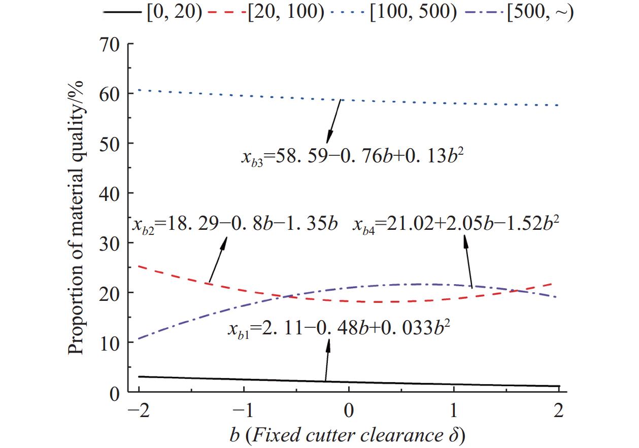
In Figure 8, the gradual increase of the gap δ raises the pass rate of materials and weakens the interaction between the cutters, which reduces the probability of producing fractured RF under external force. This might be one of the causes of the increase of the mass of RF with large outer dimension. Guillaume et al. argued that the gap between the teeth was also one of the major factors influencing the size and distribution feature of shredded thermoplastic composite material[23]. Due to the effect of various factors (thickness, pliability, and compressibility of RF), the RF shredded by cutters may be deformed and the shredding stress may be hindered[28]. The shredded films may be embedded into the gap between the cutters and S-cutter and cannot be chopped sufficiently, thus increasing the mass of the RF with large outer dimension. This change rule of gap impact is different from that of rigid plastics[23]. Khodier et al. applied different shapes of cutting tools to cut solid waste materials[17]. Their findings showed that a small gap between the cutting tool and S-cutter could reduce the passing rate of materials, while a large gap may lead to a sudden increase of materials and affect the cutting effect. Besides, with the increase of the gap δ, the interactive characteristics between the two parts would be weakened and the film stripping effect would be reduced. This may also be a cause of the increase of the mass of larger RF. Shi et al. pointed out that a smaller gap between the rake teeth and the stripping plate was better for film stripping[32]. This finding is similar to the above conclusion.
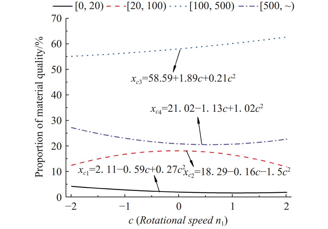
According to Figure 9, lower rotational speed of H-cutter is good for the stretching and tearing of flexible materials and can improve the cutting mass of RF. Large-torque and low-speed plastic shredding machines all adopted such a method to shred flexible materials such as plastics and woven bags[25]. If the speed discrepancy Δn between H-cutter and L-cutter is a constant value, the rotational speed n1 will increase and the rotational speed L-cutter will also increase[8]. The interaction between the two cutters would improve the stretching and tearing characteristics on RF, and the mass of excessively long RF would be reduced.
The instantaneous impact force of H-cutter increases with the increase of rotational speed n1. As RF feature good flexibility and malleability, the impact stress can be easily absorbed and hindered for effective transmission[28,33]. Rácz et al. also found that rotational speed has a large impact on the shredding probability of PET, HDPE, and textile fabrics[34]. The higher the rotational speed, the lower the stress value under a certain shredding probability. The cotton straws in MRI may shorten the time of RF layer compressing and film shredding, which is also one of the reasons why the curves of xc2 and xc3 presented an increasing trend and the xc4 curve presented a decreasing trend. Luo et al. used a saw tooth type shredding mechanism to shred urban wastes and drew the same conclusion[19,28]. When the rotational speed n1 of H-cutter increased to a certain level, RF with outside dimension larger than 500 mm were easily taken by H-cutter to S-cutter. At this time, under the interactive effect of the cutters and S-cutter, the cutting and stripping of the RF would happen simultaneously, which may be a reason why the curves of xc3 and xc4 presented an increasing trend and the xc2 curve presented a decreasing trend.
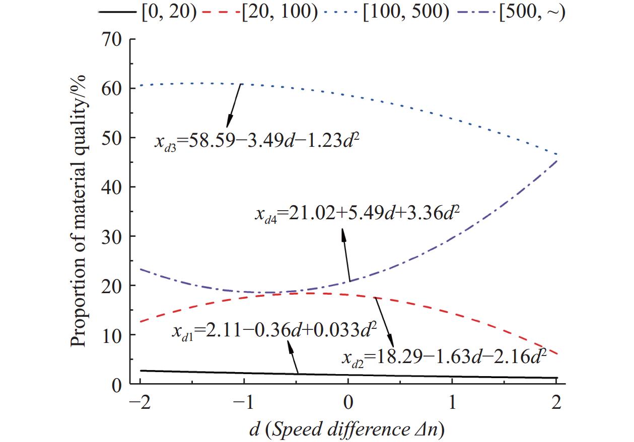
According to Figure 10, when rotational speed n1 of H-cutter is a constant value, the speed discrepancy Δn will be smaller. As the rotational speed of the L-cutter decreases, the action of the individual blades of the H-cutter becomes stronger. While this enhances the stretching, tearing, and cutting of the residual film, it also results in a weaker action of the individual blades of the H-cutter, which may contribute to the higher mass of longer RF. As Δn increased, the rotational speeds of H-cutter and L-cutter became closer and the single-roll effect of both teeth were strengthened, which may be the main reason why the xd2 curve presented an increasing trend, the xd4 curve presented a decreasing trend, and the xd3 curve gradually changed. With the rotational speeds of the H-cutter and L-cutter being close, the effectiveness of the individual rollers diminishes, resulting in less favorable conditions for stretching and tearing the RF. Consequently, this could be the primary reason for the increase in the curve of xd4 and the decrease in the curves of xd2 and xd3.
The interactive terms ab and ad are extremely significant or significant factors on test response indicator x1; bc, bd, and cd are extremely significant or significant factors on x3; bd and cd are extremely significant or significant factors on x4. Only the influence rules of extremely significant and significant factors on the test responding indicators were analyzed.
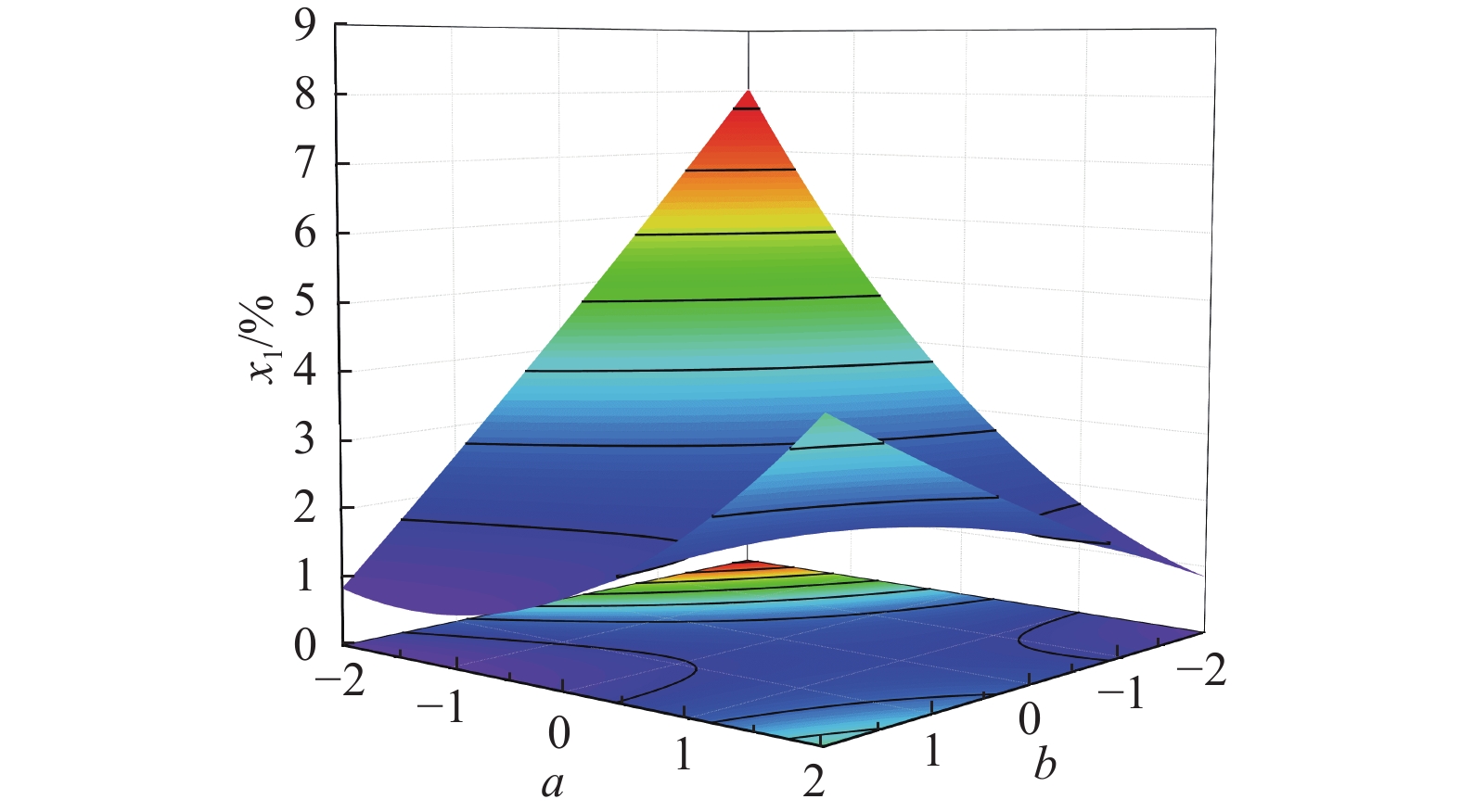
(1) Influence rule of significant interaction term ab on test response indicator x1
In Figure 11, when the level value of the test factor b is –2 and a increases from low level (–2) to high level (2), x1 presents a clear downward trend. This indicates that lower x1 can be achieved by increasing tooth number when δ is small. When the level value of the test factor b is 2 and a increases from low level (–2) to high level (2), x1 shows a tendency to decrease and then increase, and x1 reaches the minimum when the level value of b is around –1. This indicates that x1 is small under the effect of δ when tooth number is close to 6.
When the level value of the test factor a is –2 and b increases from low level (–2) to high level (2), x1 exhibits a significant downward trend. This means that for a small number of cutters, x1 can be reduced by increasing δ. When the value a is 2 and b increases from –2 to 2, x1 presents an increasing trend. This means that when tooth number is large, x1 can be effectively reduced by reducing δ. Moreover, under the dual influence of increasing both test factors a and b from –2 to 2, x1 exhibits a trend of first reduction and then increase. This trend is the same as the odd factor a influencing x1, showing that the impact of a on x1 is more obvious.
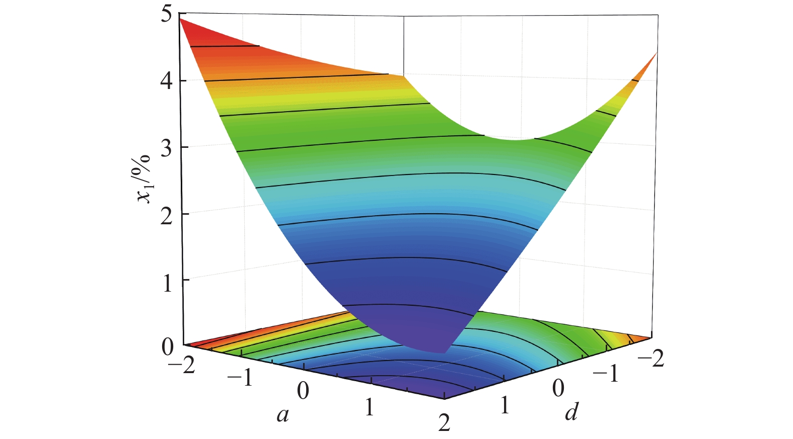
(2) Influence rule of significant interaction term ad on test response indicator x1
In Figure 12, when the level value of the test factor d is –2 and a increases from low level (–2) to high level (2), the value of x1 shows a trend of first falling and then rising, and there is a smaller x1 when tooth number is close to 8. Under the above conditions, the trend of x1 is the same as that influenced by an odd factor a. The test factor also exerts some impact on x1, but the impact is smaller than that of the odd factor a. When the level value of the test factor d is 2 and a increases from low level (–2) to high level (2), x1 shows a clear reduction trend. This trend is identical to the one influenced by an odd factor b, indicating that the value of x1 can be effectively reduced by increasing the number of teeth when Δn is –100 r/min.
When the level value of the test factor a is –2 and d increases from low level (–2) to high level (2), the value of x1 exhibits a clear increasing trend, which is contrary to the change trend of x1 influenced by the odd factor d. With a small number of cutters, the value of x1 may be effectively reduced by reducing Δn. When the level value of the test factor a is 2 and b increases from low level (–2) to high level (2), x1 shows a declining trend, which is the same effect as that of the odd factor d, which indicates that when Δn is –100 r/min, the value of x1 can be effectively reduced by increasing tooth number. With a large number of cutters, the impact of the factor d on the change trend of x1 is significant, and x1 can be reduced by increasing Δn. In addition, with the double effect of a and d both increasing from –2 to 2, the value of x1 presents a decreasing trend. This trend is the same as that of x1 influenced by odd factor d, which indicates that the impact of odd factor d on x1 is more obvious.
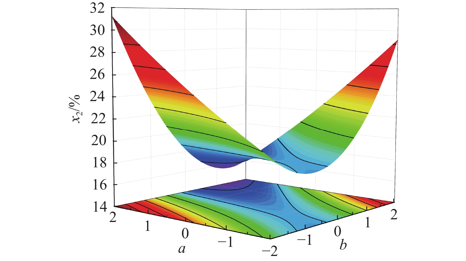
(1) Influence rule of significant interaction term ab on the test response indicator x2
In Figure 13, when factor b is –2 and a increases from low level (–2) to high level (2), the value of x2 presents a distinct increasing trend. For smaller δ, the increase of tooth number can effectively raise the value of x2. When the factor b is 2 and a increases from low level (–2) to high level (2), the value of x2 exhibits a clear reduction trend. For larger δ, the decrease of tooth number can effectively raise the value of x2.
When the level value of the test factor a is –2 and b increases from low level (–2) to high level (2), the value of x2 shows a tendency to descend first and then to rise. This tendency to vary is consistent with the tendency for the odd factors a and b to affect x2 separately. Higher x2 can be obtained when tooth number is small, whether the gap δ is large or small. The increase of x2 is more significant when tooth number is small and δ is large.
When the factor a is 2 and b increases from low level (–2) to high level (2), the value of x2 also presents a tendency to first decrease and then increase. This trend is the same as that of the odd factors a and b influencing x2, separately. Higher x2 can be obtained when tooth number is large and δ is small. Furthermore, with the double effect of test factors a and b both increasing from low level (–2) to high level (2), the value of x2 presents a decreasing trend. To prevent a decrease of x2, it is recommended to avoid simultaneously increasing the levels of both factors.
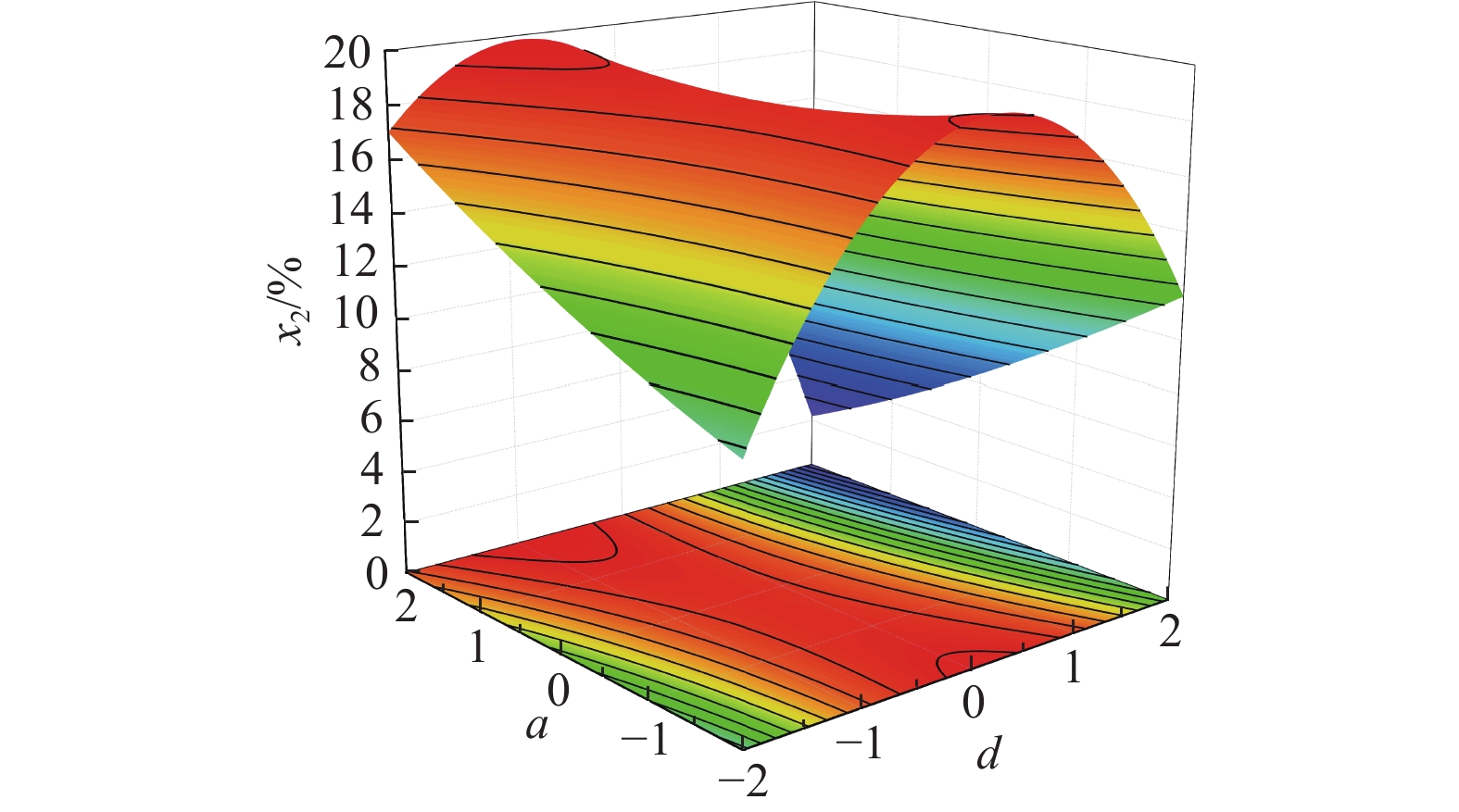
(2) Influence rule of significant interaction term ad on the test response indicator x2
In Figure 14, when the level value of the test factor d is –2 and a increases from low level (–2) to high level (2), the value of x2 presents an increasing trend. When the factor d is 2 and a increases from low level (–2) to high level (2), the value of x2 presents a decreasing trend. Therefore, the value of x2 can be effectively increased by increasing tooth number when the speed discrepancy Δn is small. For large speed discrepancy Δn, x2 can be increased by reducing tooth number.
When the factor a is –2 and d increases from low level (–2) to high level (2), the value of x2 exhibits a first increasing and then decreasing trend. When d is around 0, i.e., the speed discrepancy Δn is –300 r/min, the value of x2 is quite high. The change trend of x2 under the aforementioned conditions is consistent with that observed under the influence of the single-factor term d, and the level value of factor d corresponding to the highest x2 value is also similar. The change trend of x2 under the above-mentioned condition is identical to that influenced by the single-factor term d, and the maximum value of x2 is also close to the level value of d. This shows that the speed discrepancy Δn has significant impact on the value of x2, even with a small number of cutters.
When the factor a is 2 and d increases from low level (–2) to high level (2), the value of x2 also shows a trend of first increasing and then decreasing. When d is close to –1, i.e., the speed discrepancy Δn is close to –400 r/min, the value of x2 is quite high. The change trend of x2 under the aforementioned condition is the same as that influenced by the factor d. This shows that the speed discrepancy Δn has significant impact on the value of x2, even when tooth number is large. For a large number of cutters, the level value of the test factor corresponding to the maximum x2 drops to some extent. Meanwhile, with the double effect of test factors a and d both increasing from –2 to 2, the value of x2 exhibits a first increasing and then decreasing trend. This indicates that when both experimental factors are adjusted to near the 0 level, higher x2 values can be achieved.
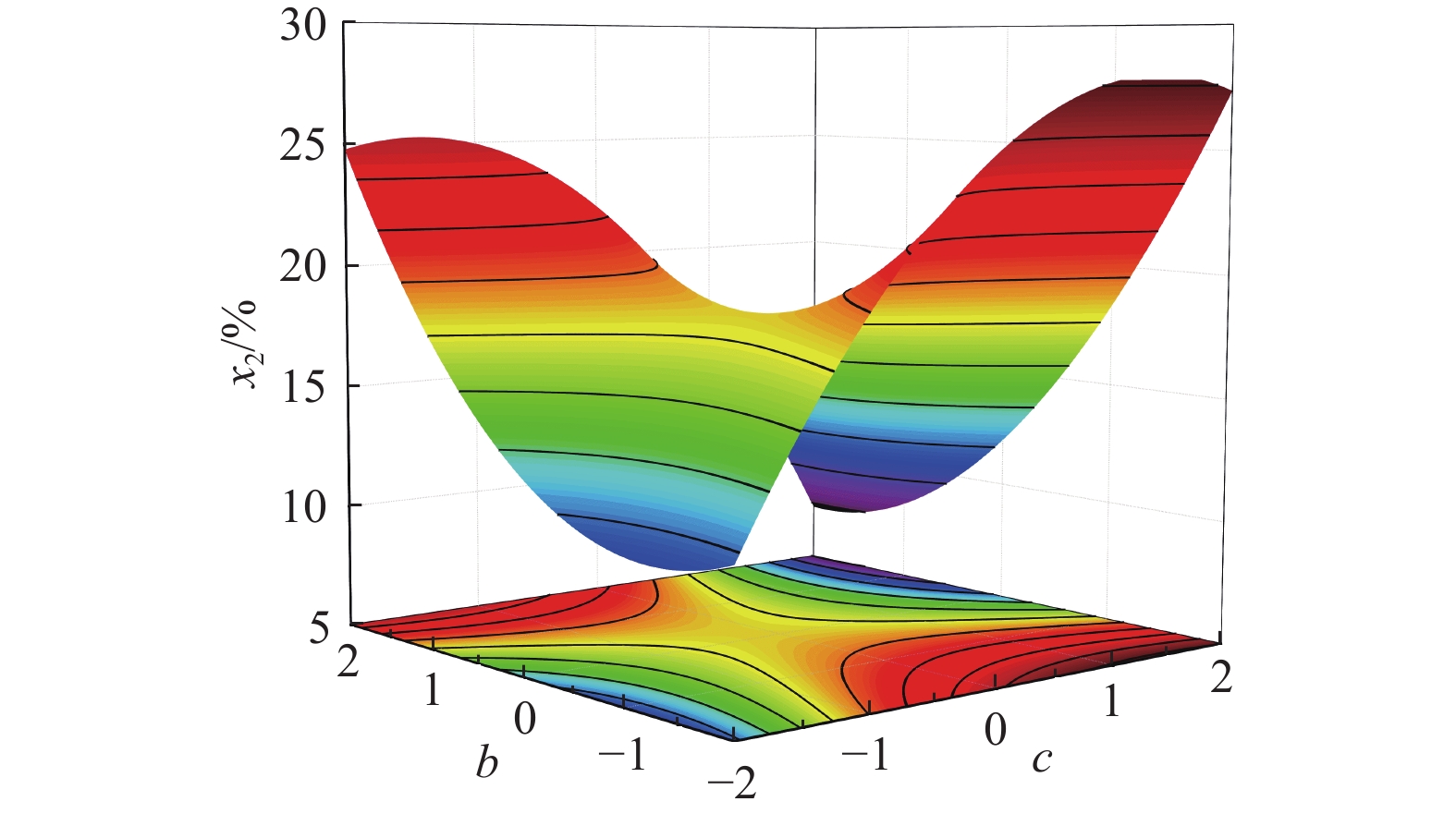
(3) Influence rule of significant interaction term bc on the test response indicator x2
In Figure 15, when the level value of the test factor c is –2 and b increases from low level (–2) to high level (2), the value of x2 presents a first decreasing and then increasing trend, and the increasing trend is more obvious. x2 is small when the gap δ is close to 2 mm. The change trend of x2 under the above condition is the same way as it is affected by the factor b. This indicates that when the rotational speed n1 is low, the gap δ has significant impact on the value of x2. Therefore, in order to obtain a higher x2 when the rotational speed n1 is low, the gap δ should be increased.
When the factor c is 2 and b increases from low level (–2) to high level (2), the value of x2 also presents a first decreasing and then increasing trend. The change trend of x2 under the above condition is the same as that influenced by the single-factor term b. This indicates that when the rotational speed n1 is high, the gap δ still has significant impact on the value of x2. Therefore, in order to obtain a higher x2 with the rotational speed n1, the gap δ should be reduced.
When the factor b is –2 and c increases from low level (–2) to high level (2), the value of x2 shows an increasing trend followed by a decreasing trend. The change trend of x2 under the above condition is the same as that influenced by the odd factor c. This means that when the gap δ is small, the rotational speed n1 still has significant impact on the value of x2. Therefore, in order to obtain a higher x2 when the gap δ is minor, higher rotational speed n1 should be used.
When the level value of the test factor b is 2 and c increases from low level (–2) to high level (2), the value of x2 presents a first increasing and then decreasing trend, and x2 is quite high when the level value of the test factor c ranges from –2 to –1. The change trend of x2 under the above condition is the same as that influenced by the odd factor c, which indicates that the rotational speed n1 has significant impact on the value of x2 when the gap δ is large. Therefore, in order to obtain a higher x2 when the gap δ is large, lower rotational speed n1 should be used. Meanwhile, with the double effect of b and c both increasing from –2 to 2, the value of x2 presents a first increasing and then decreasing trend. This trend is the same as that influenced by the odd factor c, indicating that a higher x2 can be obtained when the level values of the two test factors are adjusted close to 0.
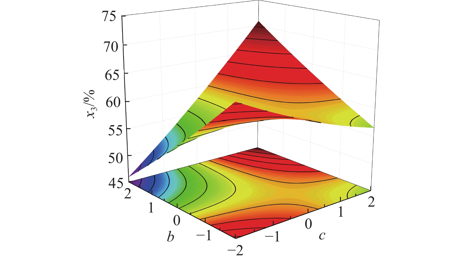
(1) Influence rule of significant interaction term bc on the test response indicator x3
In Figure 16, when the level value of the test factor c is –2 and b increases from low level (–2) to high level (2), the value of x3 presents a decreasing trend. When the factor c is 2 and b increases from low level (–2) to high level (2), the value of x3 presents an increasing trend. Therefore, the reduction of δ can help to achieve a higher x3 when n1 is low; the increase of δ can also increase x3 when n1 is high.
When the factor b is –2 and c increases from low level (–2) to high level (2), the value of x3 presents a decreasing trend. When b is 2 and c increases from low level (–2) to high level (2), the value of x3 presents an increasing trend. Therefore, the reduction of n1 can help to achieve a higher x3 when δ is small, and the increase of n1 can also raise the value of x3 when δ is large. Meanwhile, when the dual effect of test factors b and c are both increased from –2 to 2, the value of x3 exhibits a first decreasing and then increasing trend. This trend is the same as that of x3 influenced by the single-factor term b, indicating that the impact of b on the value of x3 is more obvious when the level values of the two test factors are adjusted simultaneously.
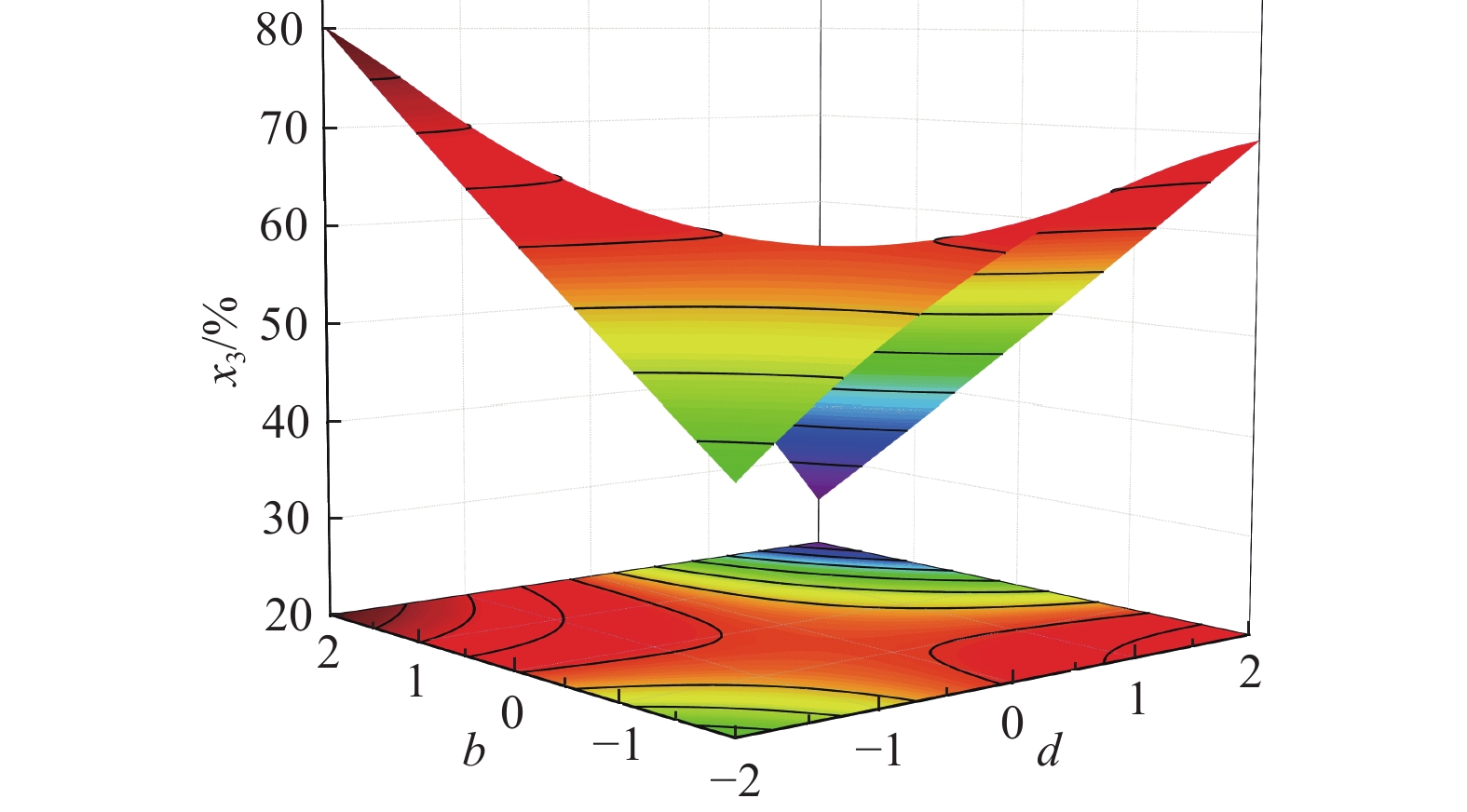
(2) Influence rule of significant interaction term bd on the test response indicator x3
In Figure 17, when the factor d is –2 and b increases from low level (–2) to high level (2), x3 presents an increasing trend. When the factor d is 2 and b increases from low level (–2) to high level (2), x3 presents a decreasing trend. Therefore, the increase of δ can help to achieve a higher x3 when Δn is small; the reduction of δ can also increase x3 when Δn is large.
When the factor b is –2 and d increases from low level (–2) to high level (2), x3 shows an increasing trend. When the level value of the test factor b is 2 and d increases from low level (–2) to high level (2), x3 presents a decreasing trend. Therefore, when δ is small, the increase of rotational speed n1 can help to achieve a higher x3. But when the gap δ is large, the reduction of n1 can also help to achieve a higher x3. In addition, with the double effect of test factors b and d both increasing from –2 to 2, the value of x3 exhibits a first increasing and then decreasing trend. This trend is the same as that of x3 influenced by the single-factor term d, and when both b and d are adjusted to near the 0 level simultaneously, higher x3 can be achieved.
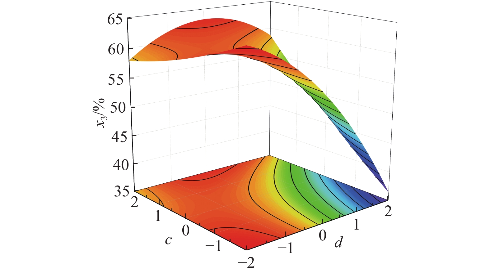
(3) Influence rule of significant interaction term cd on the test response index x3
According to Figure 18, when the factor d is –2 and c increases from low level (–2) to high level (2), x3 presents a decreasing trend. When d is 2 and c increases from low level (–2) to high level (2), x3 presents an increasing trend. Therefore, when Δn is small, the reduction of n1 can help to achieve a higher x3. But when Δn is large, increasing n1 can help to achieve a higher x3.
When the factor c is –2 and d increases from low level (–2) to high level (2), x3 presents a decreasing trend. So, when n1 is low, the reduction of Δn can help to achieve a higher x3. When the factor c is 2 and d increases from low level (–2) to high level (2), x3 presents a first increasing and then decreasing trend. When n1 is high and Δn is –300 r/min, a higher x3 can be achieved. Meanwhile, with the double effect of test factors c and d both increasing from –2 to 2, the value of x3 presents a decreasing trend. When n1 is 700 r/min and Δn is –500 r/min, a higher x3 can be achieved.
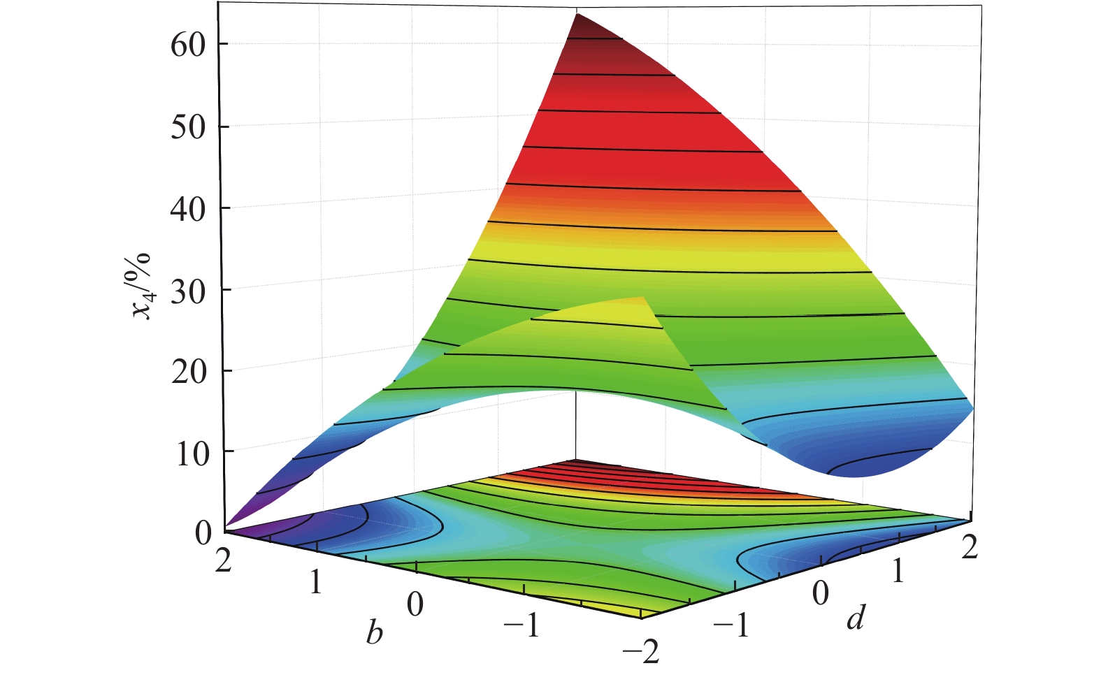
(1) Influence rule of significant interaction term bd on the test response indicator x4
In Figure 19, when the factor d is –2 and b increases from low level (–2) to high level (2), x4 performed a reducing trend. When the level value of the test factor d is 2, i.e. the speed discrepancy Δn is –100 r/min and the gap δ is gradually increased, x4 presented an increasing trend. RF with large maximum outer dimension may intertwine with cotton straws, causing trouble for the separation of MRI. Based on the above information, when Δn is small, the increase of δ can effectively reduce the mass of RF with maximum outside dimension ranged in [500, ~) mm. When Δn is high, use of smaller δ can also effectively reduce the value of x4.
When the factor b is –2 and d increases from low level (–2) to high level (2), x4 exhibits a first decreasing and then increasing trend. This trend is the same as that of x4 influenced by the single-factor term d, which indicates that Δn also has significant impact on x4 when δ is 1 mm. Based on the above information, when δ is small and Δn ranges from –300 to –200 r/min, the value of x4 is quite small.
When the level value of the test factor b is 2, i.e., the gap δ is 5 mm, x4 presents an increasing trend, and the speed discrepancy Δn also increases. When δ is large, the reduction of Δn can help to reduce the value of x4. Meanwhile, with the double effect of test factors b and d both increasing from –2 to 2, the value of x4 presents a first decreasing and then increasing trend, and there is a small level value in the range of –1 to 0. When δ is adjusted to 2-3 mm and Δn ranges from –400 to –300 r/min, a smaller x4 can be achieved.
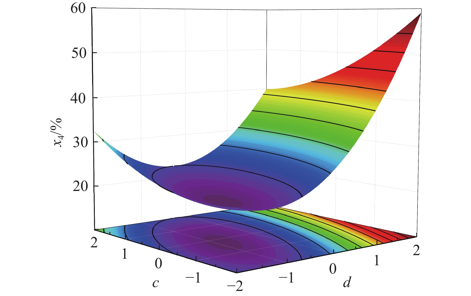
(2) Influence rule of significant interaction term cd on the test response indicator x4
In Figure 20, when the factor d is –2 and c increases from low level (–2) to high level (2), the value of x4 shows a down then up trend. The comparative analysis of the change rule of the single-factor term c affecting the value of x4 shows that the change rule of the x4 value under this condition is the same as the change rule of the single-factor term c influencing the x4 value. When the test factor d is 2, i.e., the speed discrepancy Δn is –100 r/min, x4 presents a decreasing trend. Therefore, a smaller x4 can be obtained when the speed Δn is small and the rotational speed n1 ranges from 800 to 900 r/min. When the speed Δn is large, the increase of the rotational speed n1 can help to reduce the value of x4.
When the level value of the test factor c is –2 and d increases from low level (–2) to high level (2), the value of x4 shows a trend of dropping and then rising. When the level value of the test factor c is 2, i.e., the rotational speed n1 is 1100 r/min, the value of x4 also presents a first decreasing and then increasing trend as the speed discrepancy Δn increases. According to the change rule of the single-factor term d influencing the value of x4, the change rule of x4 obtained under the above condition is the same as the change rule of the single-factor term d influencing the value of x4. Therefore, a smaller x4 can be obtained when the rotational speed n1 is small and the speed discrepancy Δn ranges from –500 to –400 r/min. The value of x4 is also small when the rotational speed n1 is small and the speed discrepancy Δn ranges from –400 to –300 r/min.
In addition, the value of x4 shows a tendency to decrease and then increase under the combined effect of increasing the test factors c and d from –2 to 2, which is the same as the change rule of the single-factor term d influencing the value of x4. According to the changes in the projection contour in the figure, a smaller x4 can be obtained when the rotational speed n1 is around 900 r/min and the speed discrepancy Δn is around –400 r/min.
Considering that the broken small RF easily caused microplastic pollution, when the outer size of the RF and the length of the cotton straw were large, it still tended to membrane straw winding. Therefore, the objective function of the maximum outer size of the RF and the size distribution of the cotton straw length was set, and the boundary conditions of the main parameters such as tooth number z (a), gap δ (b), rotational speed n1 (c), and speed discrepancy Δn (d) were constrained. The best optimized combination of main parameters of the cutting device under the given target value was obtained. The objective function value and constraint conditions were set as follows:
| {min | (13) |
In the objective function optimization process, the weight level of each experimental factor and objective function is 3+. According to the optimized results, the ideal parametric combination was: tooth number z, gap δ, rotational speed n1, and speed discrepancy Δn of 10, 2 mm, 1000 r/min, and –297.37 r/min, respectively, and the comprehensive desirability of the optimal combination parameters was 88.3% (the highest comprehensive desirability of the optimization results). Under this condition, the prediction results of each test indicator ranged from [0, 20) mm, [20, 100) mm, [100, 500) mm and [500, ~) mm and were 1.58%, 22.22%, 61.04%, 15.17%. For repeated test and test results statistics, refer to Sections 3.1 and 3.2. The prediction results of each test indicator ranged from [0, 20) mm, [20, 100) mm, [100, 500) mm and [500, ~) mm and were (1.68±0.51)%, (21.29±4.09)%, (60.41±4.52)% and (16.62±4.73)%, separately. The errors between the physical test value and model predictions were 6.33%, 4.19%, 1.03%, and 9.56%, separately, and the mean value was 5.28%. This indicates that the experimental validation results are generally consistent with the model predictions.
1) The stress characteristics of RF material layer under the conditions of H-cutter and L-cutter and their interaction with fixed cutters were evaluated, and the influence rule of RF dynamic properties in the cutting process of MRI was revealed.
2) Physical test results were analyzed using regression analysis of variance method to obtain the significance of the main parameters of cutting device influencing the distribution feature of RF. The influence of main parameters on the distribution feature of RF and their significant interaction were analyzed.
3) The best parameter combination obtained was: tooth number z, gap δ, rotational speed n1, and speed discrepancy Δn of 10, 2 mm, 1000 r/min, and –297.37 r/min, respectively. The error between the verified value and predicted value ranged from 1.03%-9.56%, and the mean value was 5.28%.
This paper was carried out with the National Natural Science Foundation of China (Grant No. 52475243), the National Natural Science Foundation of Shandong (Grant No. ZR2023ME209), Scientific Research Fund Project of Dezhou University (Grant No. 2023xjrc205), Science and Technology Plan Project of Tiemenguan (Grant No. 2023GG2202), and Xinjiang Production and Construction Corps Science and Technology Plan Project (Grant No. 2024YD014).
| [1] |
Wang Z H, Wu Q, Fan B H, Zhang J Z, Li W H, Zheng X R, et al. Testing biodegradable films as alternatives to plastic films in enhancing cotton (Gossypium hirsutum L.) yield under mulched drip irrigation. Soil and Tillage Research, 2019; 192: 196–205.
|
| [2] |
Zou X Y, Niu W Q, Liu J J, Li Y, Liang B H, Guo L L, et al. Effects of residual mulch film on the growth and fruit quality of tomato (lycopersicon esculentum mill). Water, Air, and Soil Pollution, 2017; 228(2): 71. DOI: 10.1007/s11270-017-3255-2
|
| [3] |
Kasirajan S, Ngouajio M. Polyethylene and biodegradable mulches for agricultural applications: A review. Agronomy for Sustainable Development, 2012; 32(2): 501–529. DOI: 10.1007/s13593-011-0068-3
|
| [4] |
He H J, Wang Z H, Guo L, Zheng X R, Zhang J Z, Li W H, et al. Distribution characteristics of residual film over a cotton field under long-term film mulching and drip irrigation in an oasis agroecosystem. Soil & Tillage Research, 2018; 180: 194–203.
|
| [5] |
Zhang Y L, Wang F X, Shock C C, Yang K J, Kang S Z, Qin J T, et al. Influence of different plastic film mulches and wetted soil percentages on potato grown under drip irrigation. Agricultural Water Management, 2017; 180: 160–171. DOI: 10.1016/j.agwat.2016.11.018
|
| [6] |
Li Y Q, Zhao C X, Yan C R, Mao L L, Liu Q, Li Z, et al. Effects of agricultural plastic film residues on transportation and distribution of water and nitrate in soil. Chemosphere, 2020; 242: 125131. DOI: 10.1016/j.chemosphere.2019.125131
|
| [7] |
Yang S M, Yan L M, Mo Y S, Chen X G, Zhang H M, Jiang D L. Design and experiment on collecting device for profile modeling residual plastic film collector. Transactions of the CSAM, 2018; 49(12): 109–115, 164. (in Chinese) DOI: 10.6041/j.issn.1000-1298.2018.12.013
|
| [8] |
Liang R Q, Zhang B C, Zhou P F, Li Y P, Meng H W, Kan Z. Cotton length distribution characteristics in the shredded mixture of mechanically recovered residual films and impurities. Industrial Crops and Products, 2022; 182: 114917. DOI: 10.1016/j.indcrop.2022.114917
|
| [9] |
Möllnitz S, Khodier K, Pomberger R, Sarc R. Grain size dependent distribution of different plastic types in coarse shredded mixed commercial and urban waste. Waste Management, 2020; 103: 388–398. DOI: 10.1016/j.wasman.2019.12.037
|
| [10] |
Qu J P, Huang Z X, Yang Z T, Zhang G Z, Yin X C, Feng Y H, et al. Industrial-scale polypropylene-polyethylene physical alloying toward recycling. Engineering, 2022; 9(2): 97–102.
|
| [11] |
Pomberger R, Sarc R, Lorber K E. Dynamic visualisation of urban waste management performance in the EU using ternary diagram method. Waste Management, 2017; 61: 558–571. DOI: 10.1016/j.wasman.2017.01.018
|
| [12] |
Blanco I, Schettini E, Loisi R V, Sica C, Vox G. Agricultural plastic waste mapping using GIS: A case study in Italy. Resources, Conservation, and Recycling, 2018; 137: 229–242. DOI: 10.1016/j.resconrec.2018.06.008
|
| [13] |
Vasudevan R, Sekar A R C, Sundarakannan B, Velkennedy R. A technique to dispose waste plastics in an ecofriendly way - Application in construction of flexible pavements. Construction & Building Materials, 2012; 28(1): 311–320.
|
| [14] |
Leslie H A, Leonards P E G, Brandsma S H, Boer D J, Jonkers N. Propelling plastics into the circular economy - weeding out the toxics first. Environment International, 2016; 94: 230–234. DOI: 10.1016/j.envint.2016.05.012
|
| [15] |
Curtis A, Küppers B, Möllnitz S, Khodier K, Sarc R. Real time material flow monitoring in mechanical waste processing and the relevance of fluctuations. Waste Management, 2021; 120: 687–697. DOI: 10.1016/j.wasman.2020.10.037
|
| [16] |
Shi X, Niu C H, Qiao Y Y, Zhang H C, Wang X N. Application of plastic trash sorting technology in separating waste plastic mulch films from impurities. Transactions of the Chinese Society of Agricultural Engineering, 2016; 32(2): 22–31. (in Chinese)
|
| [17] |
Khodier K, Feyerer C, Möllnitz S, Curtis A, Sarc R. Efficient derivation of significant results from mechanical processing experiments with mixed solid waste: Coarse-shredding of commercial waste. Waste Management, 2021; 121: 164–174. DOI: 10.1016/j.wasman.2020.12.015
|
| [18] |
Liang R Q, Chen X G, Zhang B C, Meng H W, Jiang P, Peng X B, et al. Problems and countermeasures of recycling methods and resource reuse of residual film in cotton fields of Xinjiang. Transactions of the Chinese Society of Agricultural Engineering, 2019; 35(16): 1–13. (in Chinese)
|
| [19] |
Luo S Y, Xiao B, Xiao L. A novel shredder for urban solid waste (MSW): Influence of feed moisture on breakage performance. Bioresource Technology, 2010; 101(15): 6256–6258. DOI: 10.1016/j.biortech.2010.02.067
|
| [20] |
Feil A, Coskun E, Bosling M, Kaufeld S, Pretz T. Improvement of the recycling of plastics in lightweight packaging treatment plants by a process control concept. Waste Management & Research, 2019; 37(2): 120–126.
|
| [21] |
Pelkey S A, Valsangkar A J, Landva A. Shear displacement dependent strength of urban solid waste and its major constituent. Geotechnical testing journal, 2001; 24(4): 381–390. DOI: 10.1520/GTJ11135J
|
| [22] |
Xu Y F, Zhang X L, Wu S, Chen C, Wang J Z, Yuan S Q, et al. Numerical simulation of particle motion at cucumber straw grinding process based on EDEM. Int J Agric & Biol Eng, 2020; 13(6): 227–235. DOI: 10.25165/j.ijabe.20201306.5452
|
| [23] |
Guillaume A V, Bruijn T A D, Wijskamp S, Rasheed M I A, Drongelen M V, Akkerman R. Shredding and sieving thermoplastic composite scrap: Method development and analyses of the fibre length distributions. Composites Part B: Engineering, 2019; 176: 107197. DOI: 10.1016/j.compositesb.2019.107197
|
| [24] |
Liang R Q, Zhang B C, Zhou P F, Li Y P, Meng H W, Kan Z. Power consumption analysis of the multi-edge toothed device for shredding the residual film and impurity mixture. Computers and Electronics in Agriculture, 2022; 196: 106898.
|
| [25] |
Maisel F, Chancerel P, Dimitrova G, Emmerich J, Nissen N F, Schneider-Ramelow M. Preparing WEEE plastics for recycling - how optimal particle sizes in pre-processing can improve the separation efficiency of high quality plastics. Resources, Conservation, and Recycling, 2020; 154: 104619. DOI: 10.1016/j.resconrec.2019.104619
|
| [26] |
Turner T A, Pickering S J, Warrior N A. Development of recycled carbon fibre moulding compounds - preparation of waste composites. Composites, 2011; 42(3): 517–525. DOI: 10.1016/j.compositesb.2010.11.010
|
| [27] |
Jambeck J R, Geyer R, Wilcox C, Siegler T R, Perryman M, Andrady A, et al. Plastic waste inputs from land into the ocean. Science, 2015; 347(6223): 768–771. DOI: 10.1126/science.1260352
|
| [28] |
Luo S Y, Xiao B, Hu Z Q, Liu S M, Guo X J. An experimental study on a novel shredder for urban solid waste (MSW). International Journal of Hydrogen Energy, 2009; 34(3): 1270–1274. DOI: 10.1016/j.ijhydene.2008.11.057
|
| [29] |
Wang M Y, Song W D, Xiao H R, Ren C H, Li S K. Design and experiment of 9MF-720 cotton stalk shredder. Journal of Agricultural Mechanization Research, 2012; 34(11): 94–96, 101. (in Chinese)
|
| [30] |
Shinners K J, Jirovec A G, Shaver R D, Bal M. Processing whole-plant corn silage with crop processing rolls on a pull-type forage harvester. Applied Engineering in Agriculture, 2000; 16(4): 323–331. DOI: 10.13031/2013.5214
|
| [31] |
Xue Z, Fu J, Chen Z, Wang F D, Han S P, Ren L Q. Optimization experiment on parameters of chopping device of forage maize harvester. Journal of Jilin University (Engineering and Technology Edition), 2020; 50(2): 739–748. (in Chinese)
|
| [32] |
Shi L L, Hu Z C, Gu F W, Wu F, Chen Y Q. Design on automatic unloading mechanism for teeth type residue plastic film collector. Transactions of the Chinese Society of Agricultural Engineering, 2017; 33(18): 11–18. (in Chinese)
|
| [33] |
Sakai S, Sawell S E, Chandler A J, Eighmy T T, Kosson D S, Vehlow J, et al. World trends in urban solid waste management. Waste Management, 1996; 16(5): 341.
|
| [34] |
Rácz Á, Csőke B. Comminution of single real waste particles in a swing-hammer shredder and axial gap rotary shear. Powder Technology, 2021; 390: 182. DOI: 10.1016/j.powtec.2021.05.064
|
Figures(20) / Tables(2)


Supported by: Beijing Renhe Information Technology Co., Ltd. 
| No. | a | b | c | d | x1/% | x2 /% | x3/% | x4/% |
| 1 | –1 (6) | –1 (2 mm) | –1 (800 r·min–1) | –1 (–400 r·min–1) | 5.68±1.52 | 16.29±3.06 | 59.56±3.09 | 18.47±3.87 |
| 2 | 1 (10) | –1 | –1 | –1 | 2.45±0.88 | 18.15±7.28 | 57.42±6.26 | 21.98±10.42 |
| 3 | –1 | 1 (4 mm) | –1 | –1 | 2.67±0.55 | 17.91±4.21 | 67.49±4.06 | 11.93±6.65 |
| 4 | 1 | 1 | –1 | –1 | 4.56±1.48 | 18.99±7.04 | 64.37±5.07 | 12.08±4.08 |
| 5 | –1 | –1 | 1 (1000 r·min–1) | –1 | 3.19±1.88 | 18.16±10.10 | 60.80±8.15 | 17.85±6.88 |
| 6 | 1 | –1 | 1 | –1 | 2.87±1.47 | 23.65±17.64 | 54.36±18.35 | 19.12±18.24 |
| 7 | –1 | 1 | 1 | –1 | 1.85±0.25 | 16.54±4.04 | 70.19±3.94 | 11.42±3.94 |
| 8 | 1 | 1 | 1 | –1 | 2.43±0.53 | 14.61±5.37 | 66.78±7.06 | 16.18±10.24 |
| 9 | –1 | –1 | –1 | 1 (–200 r·min–1) | 5.44±2.20 | 11.84±6.10 | 59.12±6.29 | 23.60±2.80 |
| 10 | 1 | –1 | –1 | 1 | 2.13±0.67 | 14.61±8.60 | 62.93±9.99 | 20.33±14.99 |
| 11 | –1 | 1 | –1 | 1 | 2.02±0.58 | 20.82±3.78 | 44.65±5.76 | 32.51±8.47 |
| 12 | 1 | 1 | –1 | 1 | 1.57±0.29 | 12.78±5.88 | 40.49±3.53 | 45.16±6.23 |
| 13 | –1 | –1 | 1 | 1 | 3.36±1.99 | 18.26±6.16 | 59.75±8.25 | 18.63±9.31 |
| 14 | 1 | –1 | 1 | 1 | 1.45±0.43 | 18.31±5.36 | 64.69±6.69 | 15.55±3.23 |
| 15 | –1 | 1 | 1 | 1 | 1.65±0.88 | 14.13±5.78 | 59.02±2.36 | 25.2±6.78 |
| 16 | 1 | 1 | 1 | 1 | 1.47±0.28 | 9.16±3.11 | 56.52±5.70 | 32.85±3.93 |
| 17 | –2 (4) | 0 (3 mm) | 0 (900 r·min–1) | 0 (–300 r·min–1) | 4.39±2.16 | 18.78±7.67 | 62.57±6.50 | 14.26±8.91 |
| 18 | 2 (12) | 0 | 0 | 0 | 2.11±1.15 | 17.25±7.65 | 63.51±11.98 | 17.13±8.29 |
| 19 | 0 (8) | –2 (1 mm) | 0 | 0 | 2.97±1.14 | 24.15±7.79 | 60.82±3.12 | 12.06±10.20 |
| 20 | 0 | 2 (5 mm) | 0 | 0 | 1.33±0.32 | 21.66±11.70 | 56.25±6.44 | 20.76±6.02 |
| 21 | 0 | 0 | –2 (700 r·min–1) | 0 | 4.58±2.29 | 12.83±8.18 | 56.55±8.09 | 26.04±12.03 |
| 22 | 0 | 0 | 2 (1100 r·min–1) | 0 | 1.58±0.59 | 10.17±4.59 | 61.15±7.31 | 27.10±8.99 |
| 23 | 0 | 0 | 0 | –2 (–500 r·min–1) | 2.68±0.96 | 12.56±8.66 | 60.55±7.87 | 24.21±10.74 |
| 24 | 0 | 0 | 0 | 2 (–100 r·min–1) | 1.62±0.63 | 5.14±2.54 | 45.58±13.75 | 47.66±15.84 |
| 25 | 0 | 0 | 0 | 0 | 1.57±0.89 | 18.78±4.25 | 56.83±4.80 | 22.82±8.07 |
| 26 | 0 | 0 | 0 | 0 | 2.60±0.42 | 18.90±6.79 | 55.55±4.91 | 22.95±7.20 |
| 27 | 0 | 0 | 0 | 0 | 1.75±0.36 | 20.02±4.34 | 59.38±5.64 | 18.85±8.18 |
| 28 | 0 | 0 | 0 | 0 | 2.19±0.64 | 17.39±3.47 | 62.10±8.04 | 18.32±6.75 |
| 29 | 0 | 0 | 0 | 0 | 2.34±0.40 | 19.58±13.17 | 55.76±5.54 | 22.32±13.61 |
| 30 | 0 | 0 | 0 | 0 | 2.22±0.64 | 15.04±7.17 | 61.91±8.89 | 20.83±15.38 |
DownLoad:
CSV
| Source | x1 | x2 | x3 | x4 | ||||||||||
| F-Value | p-value | F-Value | p-value | F-Value | p-value | F-Value | p-value | |||||||
| Model | 8.66 | <0.0001** | 11.21 | <0.0001** | 10.04 | <0.0001** | 14.19 | <0.0001** | ||||||
| a | 18.1 | 0.0007** | 0.63 | 0.4392 | 0.67 | 0.4257 | 3.6 | 0.0771 | ||||||
| b | 18.54 | 0.0006** | 5.17 | 0.0381* | 1.8 | 0.1995 | 10.1 | 0.0062** | ||||||
| c | 27.84 | <0.0001** | 0.21 | 0.6535 | 11.08 | 0.0046** | 3.07 | 0.0999 | ||||||
| d | 10.45 | 0.0056** | 21.33 | 0.0003** | 37.89 | <0.0001** | 72.39 | <0.0001** | ||||||
| ab | 23.15 | 0.0002** | 12.01 | 0.0035** | 1.45 | 0.2477 | 4.49 | 0.0512 | ||||||
| ac | 2.2 | 0.1588 | 0.02 | 0.8906 | 0.026 | 0.8734 | 0.037 | 0.8495 | ||||||
| ad | 4.68 | 0.0471* | 5.79 | 0.0294* | 2.4 | 0.1424 | 0.11 | 0.7407 | ||||||
| bc | 0.41 | 0.5322 | 23.4 | 0.0002** | 9.89 | 0.0067** | 0.049 | 0.8277 | ||||||
| bd | 1.84 | 0.1952 | 0.089 | 0.7694 | 55.16 | <0.0001** | 43.57 | <0.0001** | ||||||
| cd | 0.66 | 0.4296 | 0.068 | 0.7976 | 7.05 | 0.018* | 5.44 | 0.034* | ||||||
| a2 | 8.57 | 0.0104* | 0.16 | 0.6962 | 5.65 | 0.0312* | 7.95 | 0.013* | ||||||
| b2 | 0.1 | 0.7566 | 16.74 | 0.001** | 0.064 | 0.8034 | 6.36 | 0.0234* | ||||||
| c2 | 6.37 | 0.0233* | 20.45 | 0.0004** | 0.16 | 0.6934 | 2.85 | 0.1122 | ||||||
| d2 | 0.1 | 0.7566 | 42.55 | < 0.0001** | 5.41 | 0.0345* | 31.01 | <0.0001** | ||||||
| Lack of fit | 2.61 | 0.1506 | 0.85 | 0.6121 | 0.81 | 0.6409 | 3.12 | 0.1106 | ||||||
| R2=0.8899;R_{\rm adj}^2 =0.7871;C.V=21.01% | R2=0.9127;R_{\rm adj}^2 =0.8313;C.V=10.48% | R2=0.9036;R_{\rm adj}^2 =0.8135;C.V=4.72% | R2=0.9298;R_{\rm adj}^2 =0.8643;C.V=14.4% | |||||||||||
| Notes: ** refers to extremely significant factor (p≤0.01), *refers to significant factor (0.01<p≤0.05),p>0.05 refers to non-significant factor. | ||||||||||||||
DownLoad:
CSV

 DownLoad: